Difference-in-Differences

Introduction

• Credibility without Experimens:
  • Even without a randomized experiment, we can sometimes generate credible estimates of casual relationships in other ways.
    • Controlling for Enough
    • Natural Experiments
    • Within-unit changes
• Within-unit changes
  • Suppose we want to know the effect of a policy
  • We can find states that switched their policies, and measure trends in the outcome of interest before and after the policy change.
  • Source of Credibility:
    • Assumption: Trends in potential outcomes ($Y_0$'s and $Y_1$'s) are the same for
      • the units that did change their policy (treated)
      • the units that didn't change their policies (control)
    • Then, we have an Apples-to-Apples comparison
      • Analysis can give us credible estimate
    • This assumption is called the parallel trends assumption
      • It may be defensible/testable
      • It will be much more defensible than simply assuming that places with and without the policy are comparable.

Example and Graphical Approach

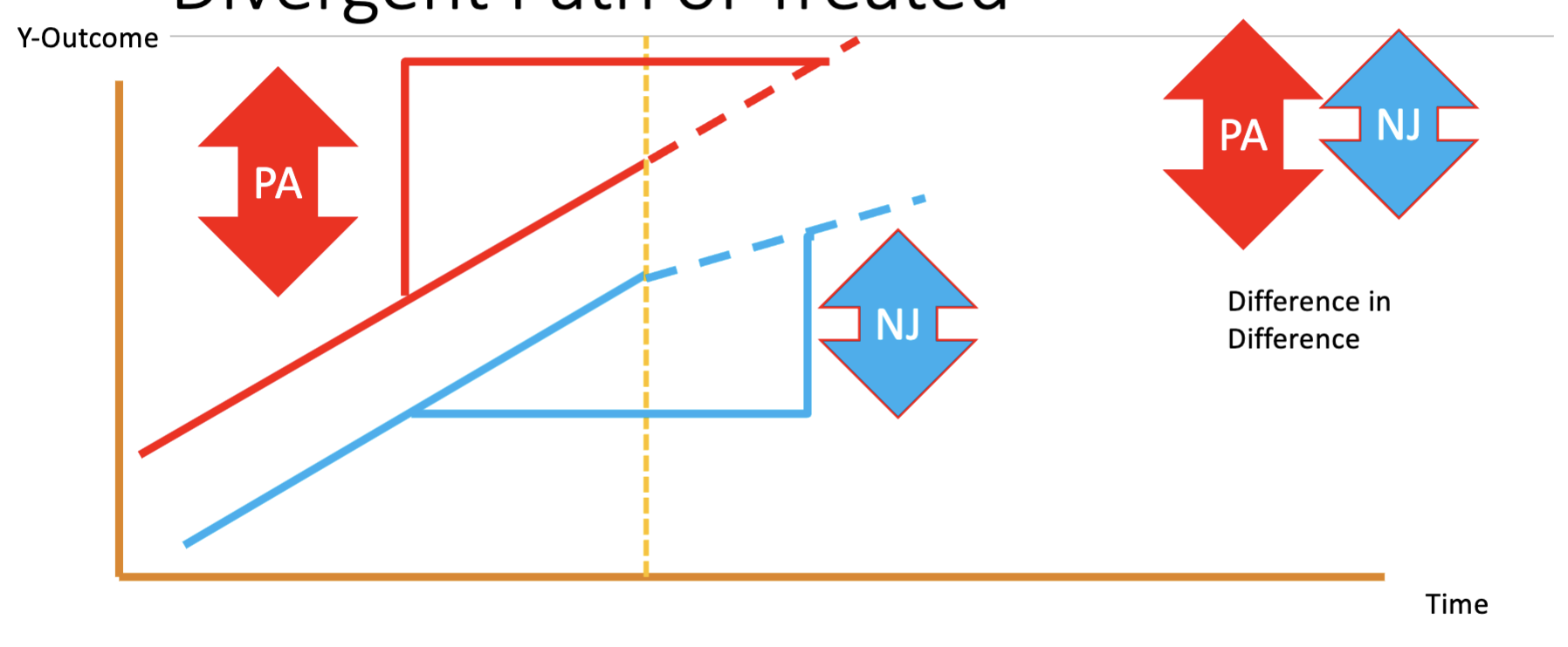
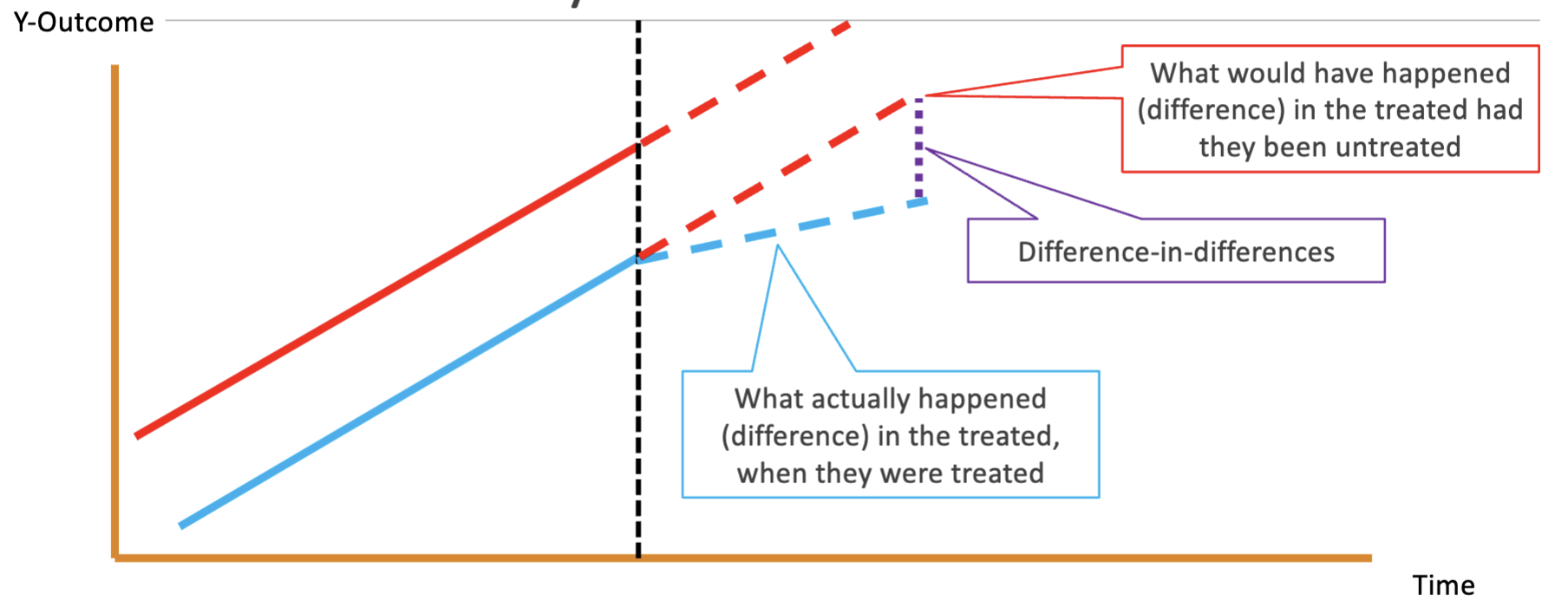
• Graphical Depiction:
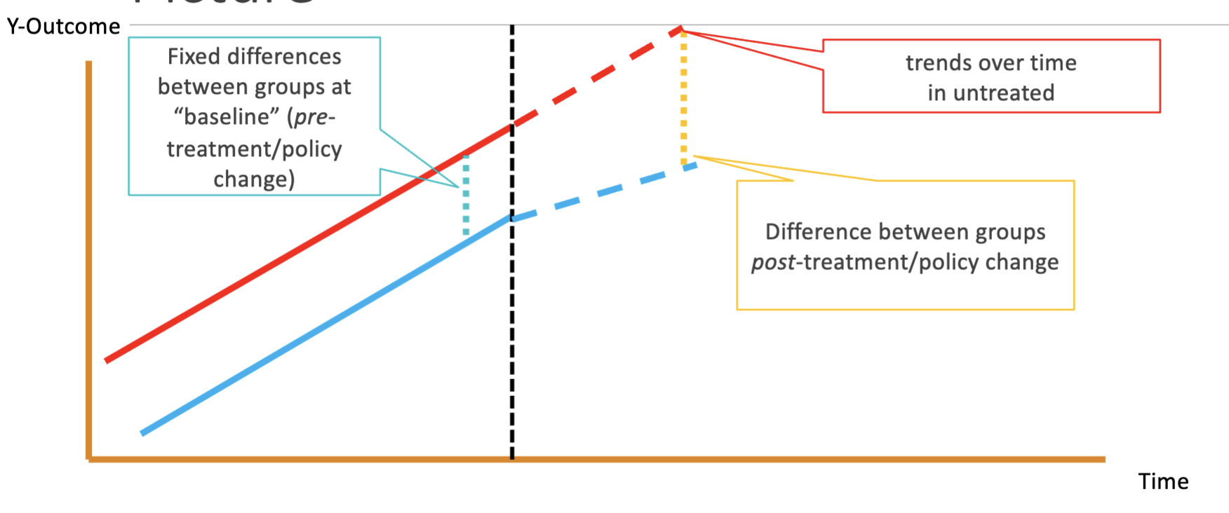
  • We compare the difference in differences between groups before and after treatment/policy change
  • Other interpretation:
    • 
    • 

Assumptions and Bias

• 2 Units and 2 Periods - Two Flawed Approaches
  • Compare the treated and untreated unit in the second period.
    • Requires the assumption that $Y_{0_\text{treated}}=Y_{0_\text{untreated}}$, which is likely unjustifiable
  • Examine the change in the outcome in the treated unit before and after the treatment.
    • Requires the assumption that nothing happened between the two periods that could have influenced the outcome (i.e., $Y_{0_\text{treated},t=2}=Y_{0_\text{treated},t=1}$), which is almost surely unjustifable in any interesting setting.
  • 2 Units and 2 Periods - Combined Approached:
    • Calculate the difference-in-differences: change in treated before and after minus change in untreated before and after $(Y_{1_\text{treated}, t=2}-Y_{0_\text{treated},t=1})-(Y_{0_\text{untreated},t=2}-Y_{0_\text{untreated},t=1})$
    • Algebraically identical to another difference-in-differences: the difference between the treated and untreated units after the treatment minus the difference between the treated and untreated units before the treatment $(Y_{1_\text{treated}, t=2}-Y_{0_\text{untreated},t=2})-(Y_{0_\text{treated},t=1} - Y_{0_\text{untreated},t=1})$
• DiD and Treatment Effects:
  • Bias: $\begin{aligned} \text{Bias}&=\text{Did}-\text{ATT}\\ &=(Y_{1_\text{treated}, t=2}-Y_{0_\text{treated},t=1})-(Y_{0_\text{untreated},t=2}-Y_{0_\text{untreated},t=1})-(Y_{1\text{treated},t=2}-Y_{0\text{treated},t=2})\\ &=(Y_{0_\text{treated},t=2}-Y_{0_\text{treated},t=1})-(Y_{0_\text{untreated},t=2}-Y_{0_\text{untreated},t=1}) \end{aligned}$
    • The DiD estimate will be biased if the change in $Y_0$'s for the treated unit differ from the change in $Y_0$'s for the untreated unit.
    • The DiD estimate is unbiased if the treated and untreated units experience the same trends in $Y_0$ (parallel treads).
  • Assumption:
    • Note that parallel trends assumptions are about $Y_0$'s or $Y_1$'s but not $Y$'s, so in this sense, the trends are fundamentally unobservable and this assumption cannot be directly tested.
• What's good about DiD?
  • DiD accounts for all time-invariant differences between units that would plague a cross-sectional analysis
  • It also accounts for all of the time-specific factors that would plague a "before-and-after" analysis
  • It does not account for time-variant differences between units.
    • This is only a problem if these factors vary in ways that correspond with the treatment.

Extending Model and Alternative Approach

• N Units and 2 Periods:
  • At least three options (all of which are algebraically identical) for calculating DiD
  • With 2 periods, all the these approaches are equivalent.
    • Approach 1: calculate the 4 means of interest (average $Y$ for treated before, average $Y$ for treated after, etc.), and calculate the DiD by hand.
    • Approach 2: Put the data into long format with 1 row per unit-period, and run the following regression: $Y_\text{it}=\beta\times T_\text{it}+\gamma_i+\delta_t+\epsilon_\text{it},$ where $\gamma_i$ represents unit fixed effects, and $\delta_t$ represents time period fixed effects.
• N Units and N periods:
  • The fixed effects approach is best here and also more flexible.
    • E.g., it allows we to include time-varying covariates