15 Clustering
Clustering
Unsupervised Learning
K-means
This lecture discusses the basics of clustering, focusing on the k-means algorithm. It covers the algorithm’s initialization, convergence, and the concept of local minima.
- Input: dataset of feature vectors \(D=\qty{\va x^{(i)}}_{i=1}^N\), where \(\va x^{(i)}\in\R^d\). We don’t have labels!
- Output: a set of clusters \(C_1,\dots,C_k\)
- Types of clusters: partitional vs. hierarchical
Partitional Clustering
- Basic idea: group similar points.
- Goal: Given a set of examples \(D=\qty{\va x^{(i)}}_{i=0}^N\), \(\va x^{(i)}\in\R^d\).
- Assign similar points to the same clusters, and
- Assign dissimilar points to different clusters.
- Measure dissmilarity: Euclidean distance: \[\norm{\va x^{(i)}-\va x^{(j)}}^2.\]
- Notation:
- \(C\): cluster, a set of point indices
- \(\va z^{(j)}\): representative example, cluster centroid.
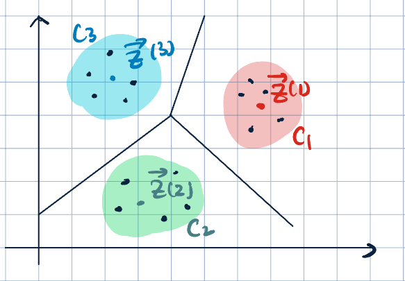
- Partition \(\R^d\) into \(k\) convex cells.
- \(z_j=\dfrac{1}{\abs{C_j}}\sum_{i\in C_j}\va x^{(i)}\).
- \(C_j=\qty{i=1,\dots,N,\quad\text{where the closest representative example to }\va x^{(i)}\text{ is }\va z^{(j)}}\)
- Given \(C_j\), we can find \(z_j\), and vice versa.

- Objective: Intertia/Within-Cluster Sum of Square/Intra-Cluster Distance \[
\min_{\textcolor{blue}{\substack{C_1,\dots,C_k\\\va z^{(1)},\dots,\va z^{(k)}}}}\textcolor{red}{\sum_{j=1}^k}\textcolor{teal}{\sum_{i\in C_j}}\norm{\va x^{(i)}-\va z^{(j)}}^2
\]
- \(\dsst\min_{\textcolor{blue}{\substack{C_1,\dots,C_k\\\va z^{(1)},\dots,\va z^{(k)}}}}\): Find clusters and their centroids.
- \(\dsst\textcolor{red}{\sum_{j=1}^k}\): Sum over all clusters.
- \(\dsst\textcolor{teal}{\sum_{i\in C_j}}\): Sum over points in each cluster.
- This problem is NP-hard.
- We have efficient heuristics to find local optimum.
\begin{algorithm} \caption{K-Means Clustering (Alternating Minimization)} \begin{algorithmic} \State{Initialize $\va z^{(1)},\dots,\va z^{(k)}$ randomly.} \While{not converged} \For{$j=1,\dots,k$} \State{$C_j=\qty{i=1,\dots,N,\text{ where the closest representative example for }\va x^{(i)}\text{ is }\va z^{(j)}}$} \EndFor \For{$j=1,\dots,k$} \State{$\dsst\va z^{(j)}=\dfrac{1}{\abs{C_j}}\sum_{i\in C_j}\va x^{(i)}$} \EndFor \EndWhile \end{algorithmic} \end{algorithm}
Example 1 (K-Means Example)

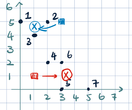
- \(k=2\)
- Initialization: \(\textcolor{blue}{\va z^{(1)}=(3,5)}\) and \(\textcolor{red}{\va z^{(2)}=(1,1)}\)
- Fix \(\va z^{(j)}\). Make assignment:
| Point | \(L^2\) Distance to \(\textcolor{blue}{\va z^{(1)}}\) | to \(\textcolor{red}{\va z^{(2)}}\) | Assignment | |
|---|---|---|---|---|
| 1 | \((0,5)\) | \(3\) | \(\sqrt{17}\) | \(\textcolor{blue}{C_1}\) |
| 2 | \((2,5)\) | \(1\) | \(\sqrt{17}\) | \(\textcolor{blue}{C_1}\) |
| 3 | \((1,4)\) | \(\sqrt{5}\) | \(3\) | \(\textcolor{blue}{C_1}\) |
| 4 | \((2,2)\) | \(\sqrt{10}\) | \(\sqrt{2}\) | \(\textcolor{red}{C_2}\) |
| 5 | \((3,0)\) | \(5\) | \(\sqrt{5}\) | \(\textcolor{red}{C_2}\) |
| 6 | \((3,2)\) | \(3\) | \(\sqrt{5}\) | \(\textcolor{red}{C_2}\) |
| 7 | \((5,0)\) | \(\sqrt{29}\) | \(\sqrt{17}\) | \(\textcolor{red}{C_2}\) |
- Update centroid:
- \(\textcolor{blue}{\va z^{(1)}=(1, 4.67)}\)
- \(\textcolor{red}{\va z^{(2)}=(3.25, 1)}\)
- We are converged already because redo the iteration will not change the assignment and clusters anymore.
- Convergence:
- Clusters/centroids stop changing.
If ties are not broken consistently, we may cycle. If it cycles, we know we converged. - \(k\)-means is guaranteed to converge (to local optimum), but we may not necessarily converge to the global optimum.
- Clusters/centroids stop changing.
- Initialization:
- Randomly
- \(k\)-means\(++\): accounts for distribution of \(\va x\) in \(\R^d\). This approach tries to “spread it out” more.
- In general, we repeat \(k\)-means multiple times. We choose clustering solution with lowest inertia.
- Choosing \(k\):
- In some applications, \(k\) will be given.
- Use validation data.
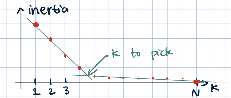
- The “elbow” method: plot inertia vs. \(k\). Choose \(k\) where the curve starts to flatten out.

Remark 1 (The Elbow Plot). If \(k=N\), every point forms its own cluster. \[\sum_{j=1}^N\sum_{i\in C_j}\norm{\va x^{(i)}-\va z^{(j)}}^2=0\implies \va z^{(j)}=\va x^{(i)}.\]