13 Reinforcement Learning
Reinforcement learning is agent-oriented learning.
The RL Interface: Sequential Decision Making
- Overfiew: At each time \(t\), the agent
- Observe state \(S_t\) (Environment)
- Executes an action \(a_t\)
- Receives a scalar reward \(r_t\)
- Transitions to the next state \(S_{t+1}\).
- The process is repeated and forms a trajectory of states, actions, and rewards: \(s_1,a_1,r_1,s_2,a_2,r_2,\dots\).
Definition 1 (Markov Decision Process (MDP))
- \(\mathcal{S}\): set of states
- \(\mathcal{A}\): set of actions
- \(R\): reward function \[p(r_t\mid s_t,a_t)\]
- \(P\): transition function \[p(s_{t+1}\mid s_t,a_t)\]
Policy: mapping from states to actions \[\pi:\mathcal{S}\to\mathcal{A}\] Goal: learn polyci that maximizes the cummulative reward: \[G=\sum_{t=1}^Tr_t.\]
Multi-Armed Bandit Problem
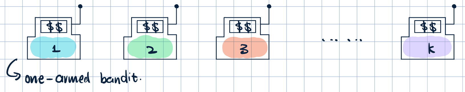
- Set-up:
\(\mathcal{S}\): single state
\(\mathcal{A}\): arms \(a=1,a=2,a=3,\dots,a=k\).
\(R\): \(P(r\mid a)\) for \(a\in\mathcal{A}\), pobablistic mapping from action to reward.
Task: Agent sequentially chooses which arm to pull next.
for steps \(t=1,\dots, T\): The arm chosed to pull: \(a_t\in\mathcal{A}\). Observed reward: \(r_t\sim P(r\mid a_t)\).
Goal: Decide a sequence of actions that maximizes cumulative reward \[\sum_{t=1}^T r_t\]
Assumption: Reward depends only on the action taken. i.e., it is i.i.d. with expectation \(\mu(a)\) for \(a=1,\dots, k\).
Example 1 (Example: Best Arm to Pull)
- action \(1\): \(\mu(a)=8\)
- action \(2\): \(\mu(a)=12\)
- action \(3\): \(\mu(a)=12.5\)
- action \(4\): \(\mu(a)=11\)
Action \(3\) is the best since \(\mu(a)\) is the highest. If we know \(\mu(a)\) for \(a\in\mathcal{A}\), then always taking \(a=3\) givesn the highest cummulative reward.
- Challenge: \(\mu(a)\) is unknown, the distribution is unknown.
Action-Value Methods
- Main idea: learn \(Q(a)\approx\mu(a)\quad\forall\,a\in\mathcal{A}\).
- Suppose we have \(a_1,r_1,a_2,r_2,\dots,a_{t-1},r_{t-1}\).
- Estimate \(\mu(a)\) for \(a\in\mathcal{A}\) as sample average: \[ \begin{aligned} Q_t(a)&=\dfrac{\text{sum of rewards when action }a\text{ is taken previously}}{\text{number of times action }a\text{ is taken previously}}\\ &=\dfrac{\dsst\sum_{i=1}^{t-1}r_1\1\qty{a_i=a}}{\dsst\underbrace{\sum_{i=1}^{t-1}\1\qty{a_i=a}}_{N_t(a)}} \end{aligned} \]
Remark 1 (Convergence of Sample Average). Sample average converges to the true value if action is taken infinitely number of times: \[ \lim_{N_t(a)\to\infty}Q_t(a)=\mu(a), \] where \(N_t(a)\) is the number of times action \(a\) has been taken by time \(t\).
Given \(Q_t(a)\) for all \(a\in\mathcal{A}\), the greedy action \(a_t^*=\argmax_{a}Q_t(a)\).
For the next action \(a_t\):
- if \(a_t=a_t^*\), we are exploiting, we kind of know which actions are good.
- if \(a_t\neq a_t^*\), we are exploring, we want to collect more data to improve estimates.
We can only pick one \(a_t\), so we can’t do both.
BUT, we have to do both.
This is the key dilemma in reinforcement learning: Exploration vs. Exploitation.
- Exploration: gain more information about value of each action.
- Exploitation: Revisit actions that are already known to given high rewards.
First attempt: Naïve approach:
- Exploration phase: Try each arm \(100\) times.
- Estimate their value as \(Q(a)\) for \(a\in\mathcal{A}\).
- Exploitation phase: Always pick \(a^*=\argmax_a Q(a)\).
- Problem:
- Is \(100\) times too much? e.g., negtive rewards \(10\) consecutive times
- Is \(100\) times enough? \(Q(a)\to\mu(a)\) in the limit of infinite samples. We should never stop exploring.
Second attempt: \(\epsilon\)-Greedy Action Selection:
- This ia simple, effective way to balance exploration and exploitation.
Remark 2 (\(\epsilon\) Controls the Exploration Rate).
- Larger \(\epsilon\), explore more, learn faster, converge to suboptimal.
- Smaller \(\epsilon\), explore less, learn slower, converge to near-optimal.
- \(\epsilon\)-greedy explores forever, and we have constant exploration rate.
- Should we explore forever?
- Yes! But perhaps explore less as time goes by.
- Key idea: “Optimism in the face of uncertainty”
- The more uncertain we are about an action, the more important it is to explore that action.
- Optimistic initialization:
- Initialize \(Q(a)\) to some positive value
- Encourage exploration initially, naturally gets “washed out” as we collect data.
- This method is somewhat hacky, but it works.
- Upper Confidence Bound (UCB) Action Selection:
- Select actions greedily based on potential of being the best
- Estimate \(Q(a)+\text{Uncertainty }N(a)\).
- UCB Score: \[Q_t(a)+c\sqrt{\dfrac{\ln(t)}{N_t(a)}},\quad c>0,\] where
- \(Q_t(a)\) is the sample average estimate
- \(\dsst c\sqrt{\dfrac{\ln(t)}{N_t(a)}}\) is the exploration bonus
- \(c\) is the degree of exploration. Larger \(c\), more exploration.
- As \(N_t(a)\) increases, more certain, explore less that action.
- As \(t\) increases, but \(N_t(a)\) doesn’t increase, explore more of that action.