9 Boosting
Goal: Reduce both approximation and estimation error at the same time (bias-variance tradeoff).
Bosting Introduction
Definition 1 (Boosting) Combine simple “weak” classifiers into a more complex “stronger” model.
- Type of boosting methos: AdaBoost and Gradient Boosting
- Weak classifier: Decision stump (a one-level decision tree)
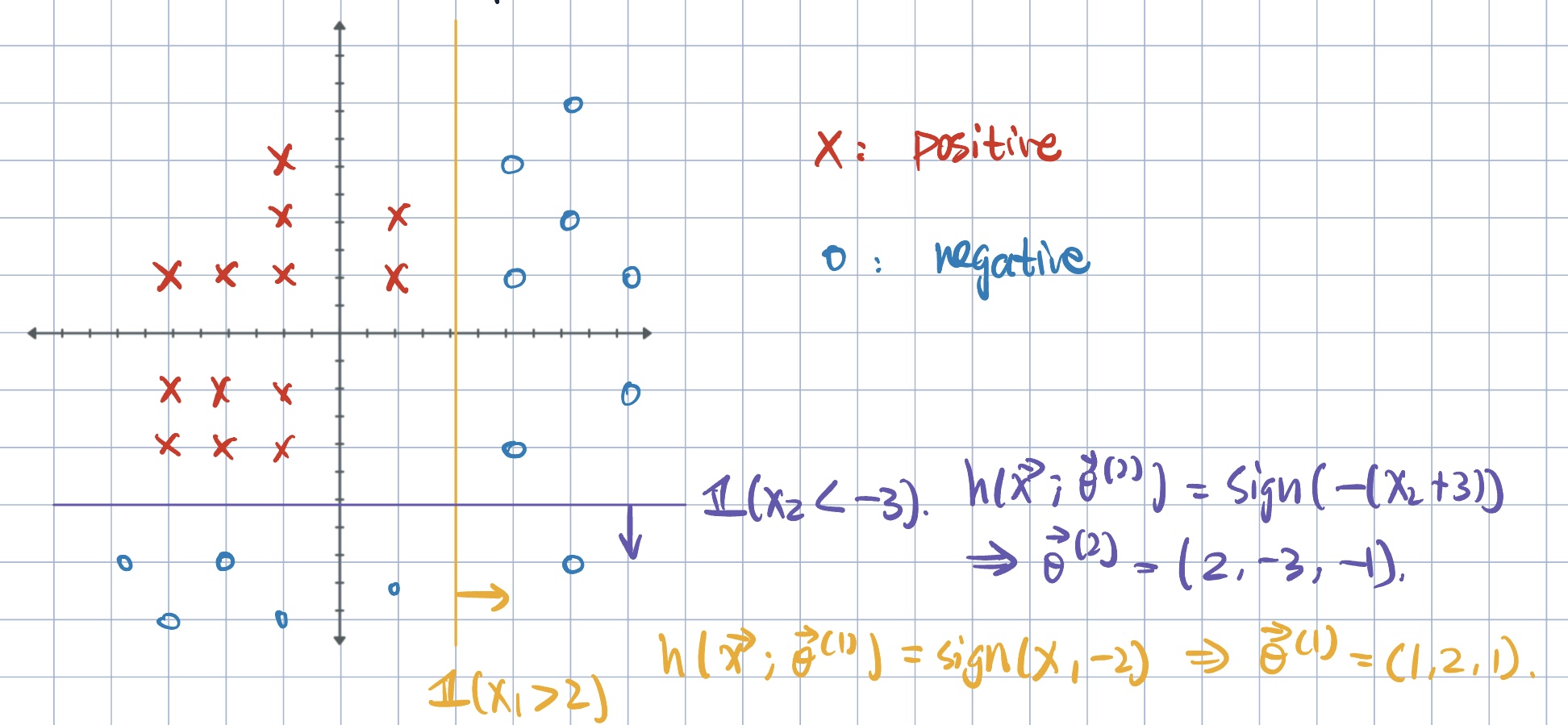
Notation: \[ h\qty(\va x;\va\theta)=\operatorname{sign}(\theta_1(x_k-\theta_0))=\pm1, \] where \(\va\theta=(k,\theta_0,\theta_1)\) such that \(k\) denotes the coordinate, \(\theta_0\) is the location, and \(\theta_1\) is the direction.
Ensemble as a weighted combination of decision stumps: \[ \begin{aligned} h_M(\va x)&=\sum_{m=1}^M\alpha_m h\qty(\va x;\va\theta^{(m)})&\text{for}\quad \alpha_m\geq0.\\ &=\alpha_1 h\qty(\va x;\va\theta^{(1)})+\alpha_2 h\qty(\va x;\va\theta^{(2)})+\cdots+\alpha_M h\qty(\va x;\va\theta^{(M)}) \end{aligned} \]
This can be viewed as a linear classifier: \(h_M(\va x)=\va\alpha\cdot\phi(\va x)\), where
- \(\phi(\va x)=\mqty[h(\va x;\va\theta^{(1)},\dots,h(\va x;\va\theta^{(M)})]\), the feature mapping
- \(\va\alpha=\mqty[\alpha_1,\dots,\alpha_m]\), the parameter vector \(\va\alpha\in\R^M\).
\(\phi(\va x)\in\R^M\):
- intead of specifying \(\phi(\va x)\), we learn \(\phi(\cdot)\) in addition to \(\va\alpha\).
- \(M\), the number of weak learners, is a hyperparameter.
AdaBoost: Adaptive Boosting
- One of the simplies and most popular boosting algorithms.
- Algorithm Overview:
- Set example weights uniformly.
- For each weak learner \(m=1,\dots, M\):
- Train decision stump on weighted examples
- Apply decision stump to all examples
- Set decision stump weight based on weighted error
- Set example weights based on ensemble predictions.
- A greedy approach: Given the current ensemble, find the next weak learner that, if added, makes a better new ensemble.
- Suppose we have the frist \((m-1)\) decision stumps, which make up an ensemble classifier \[h(\va x;\va\theta^{(1)}),\ h(\va x;\va\theta^{(2)}),\dots, h(\va x;\va\theta^{(m-1)})\implies h_{m-1}(\va x).\]
- Goal: Find the next decision stump \(h(\va x;\va\theta^{(m)})\) and its weight \(\alpha_m\) in order to minimize the same training loss (empirical risk) of the new ensemble \(h_m(\va x)\): \[ \begin{aligned} \argmin_{\va\theta^{(m)},\alpha_m} J(\alpha_m,\va\theta^{(m)})&=\argmin_{\va\theta^{(m)},\alpha_m}\sum_{i=1}^N \operatorname{loss}\qty(y^{(i)}\cdot h_m(\va x^{(i)})) &\text{exponential }\operatorname{loss}(\cdot)=e^{-z}=\exp(-z).\\ J(\alpha_m,\va\theta^{(m)})&=\sum_{i=1}^N \exp\qty(-y^{(i)}\cdot h_m(\va x^{(i)}))\\ &=\sum_{i=1}^N \exp\bigg(-y^{(i)}\bigg[\underbrace{h_{m-1}(\va x^{(i)})}_{\substack{\text{previous}\\\text{ensemble}}}+\underbrace{\alpha_mh(\va x;\va\theta^{(m)})}_{\text{update}}\bigg]\bigg)\\ &=\sum_{i=1}^N\underbrace{\exp\qty(-y^{(i)}h_{m-1}(\va x^{(i)}))}_{\substack{\text{independent of }\alpha_m,\va\theta^{(m)}\\\text{denote it as }w_{m-1}(i)}}\exp\qty(-y^{(i)}\alpha_mh(\va x;\va\theta^{(m)}))\\ &=\sum_{i=1}^N w_{m-1}(i)\exp\qty(-y^{(i)}\alpha_mh(\va x;\va\theta^{(m)}))\\ \end{aligned} \]
- Let \(w_{m-1}(i)=\exp\qty(-y^{(i)}h_{m-1}(\va x^{(i)}))\):
- Loss associated with the previous ensemble with respect to the \((i)\)-th point.
- Used as weight for each training example: \(i=1,\dots, N\).
- New decision stump \(\va\theta^{(m)}\) will be more heavily influenced by examples that were misclassified by the previous ensemble.
- Note: weighted loss associated with point \(\va x^{(i)}\) in the objective: \[ J(\alpha_m,\va\theta{(m)})=\begin{cases}w_{m-1}(i)\exp(-\alpha_m)\quad&\text{if }\va x^{(i)}\text{ is correctly classified}\\w_{m-1}(i)\exp(\alpha_m)\quad&\text{o/w}.\end{cases} \] If \(\va x^{(i)}\) is correctly classified: \(y^{(i)}=h(\va x;\va\theta^{(m)})\). Let’s normalize example weigths so that they sum to \(1\): \[ \tilde w_{m-1}(i)=\dfrac{w_{m-1}(i)}{\dsst\sum_{j} w_{m-1}(j)}. \] Then, \[ \begin{aligned} \tilde J(\alpha_m,\va\theta^{(m)})&=\underbrace{\exp(-\alpha_m)\sum_{i:y^{(i)}=h(\va x^{(i)};\va\theta^{(m)})}\tilde w_{m-1}(i)}_\text{correctly classified}+\underbrace{\exp(\alpha_m)\sum_{i:y^{(i)}\neq h(\va x^{(i)};\va\theta^{(m)})}\tilde w_{m-1}(i)}_\text{incorrect points}\\ &=\exp(-\alpha_m)\underbrace{\sum_{i=1}^N\tilde w_{m-1}(i)}_{=1}-\exp(-\alpha_m)\sum_{i=1}^N\tilde{w}_{m-1}(i)\1\qty{y^{(i)}\neq h(\va x^{(i)}\neq h(\va x^{(i);\va\theta^{(m)}}))}\\ &\qquad\qquad+\exp(\alpha_m)\sum_{i=1}^N\tilde{w}_{m-1}(i)\1\qty{y^{(i)}\neq h(\va x^{(i)};\va\theta^{(m)})}\\ &=\exp(-\alpha_m)+\underbrace{\qty\bigg(\exp(\alpha_m)-\exp(-\alpha_m))}_{\geq0}\sum_{i=1}^N\tilde{w}_{m-1}(i)\1\qty{y^{(i)}\neq h(\va x^{(i)};\va\theta^{(m)})}\\ \end{aligned} \] So, our objective is \[ \argmin_{\va\theta^{(m)},\alpha_m}\exp(-\alpha_m)+\qty\bigg(\exp(\alpha_m)-\exp(-\alpha_m))\sum_{i=1}^N\tilde{w}_{m-1}(i)\1\qty{y^{(i)}\neq h(\va x^{(i)};\va\theta^{(m)})} \]
- To solve:
- First solve for best \(\va\theta^{(m)*}\), then \[ \va\theta^{(m)*}=\argmin_{\va\theta^{(m)}}\underbrace{\sum_{i=1}^N\tilde{w}_{m-1}(i)\1\qty{y^{(i)}\neq h(\va x^{(i)};\va\theta^{(m)})}}_{\substack{\epsilon_m\text{: weighted classification error}\\\text{of decision stumps}}}=\argmin_{\va\theta^{(m)}}\,\epsilon_m \] It is easy to optimize \(\va\theta^{(m)}\) via an exhaustive search over all possible decision stumps. Denote \[ \tilde\epsilon_m=\sum_{i=1}^N\tilde{w}_{m-1}(i)\1\qty{y^{(i)}\neq h(\va x^{(i)};\va\theta^{(m)*})} \]
- Figure out how much weight to give it. \[ \alpha_m^*=\argmin_{\alpha_m}\underbrace{\exp(-\alpha_m)+\qty[\exp(\alpha_m)-\exp(-\alpha_m)]\tilde\epsilon_m}_{L(\alpha_m).} \] By FOC: \[ \begin{aligned} \dfrac{\partial L(\alpha_m)}{\partial\alpha_m}=-\exp(-\alpha_m)+\qty[\exp(\alpha_m)-\exp(-\alpha_m)]\tilde\epsilon_m&\overset{\text{set}}{=}0\\ (\epsilon_m-1)\exp(-\alpha_m)+\epsilon_m\exp(\alpha_m)&=0\\ \implies\alpha_m^*&=\dfrac{1}{2}\ln\dfrac{1-\tilde\epsilon_m}{\tilde\epsilon_m}\\ \end{aligned} \]
Example 1 (How AdaBoost Works in Action)
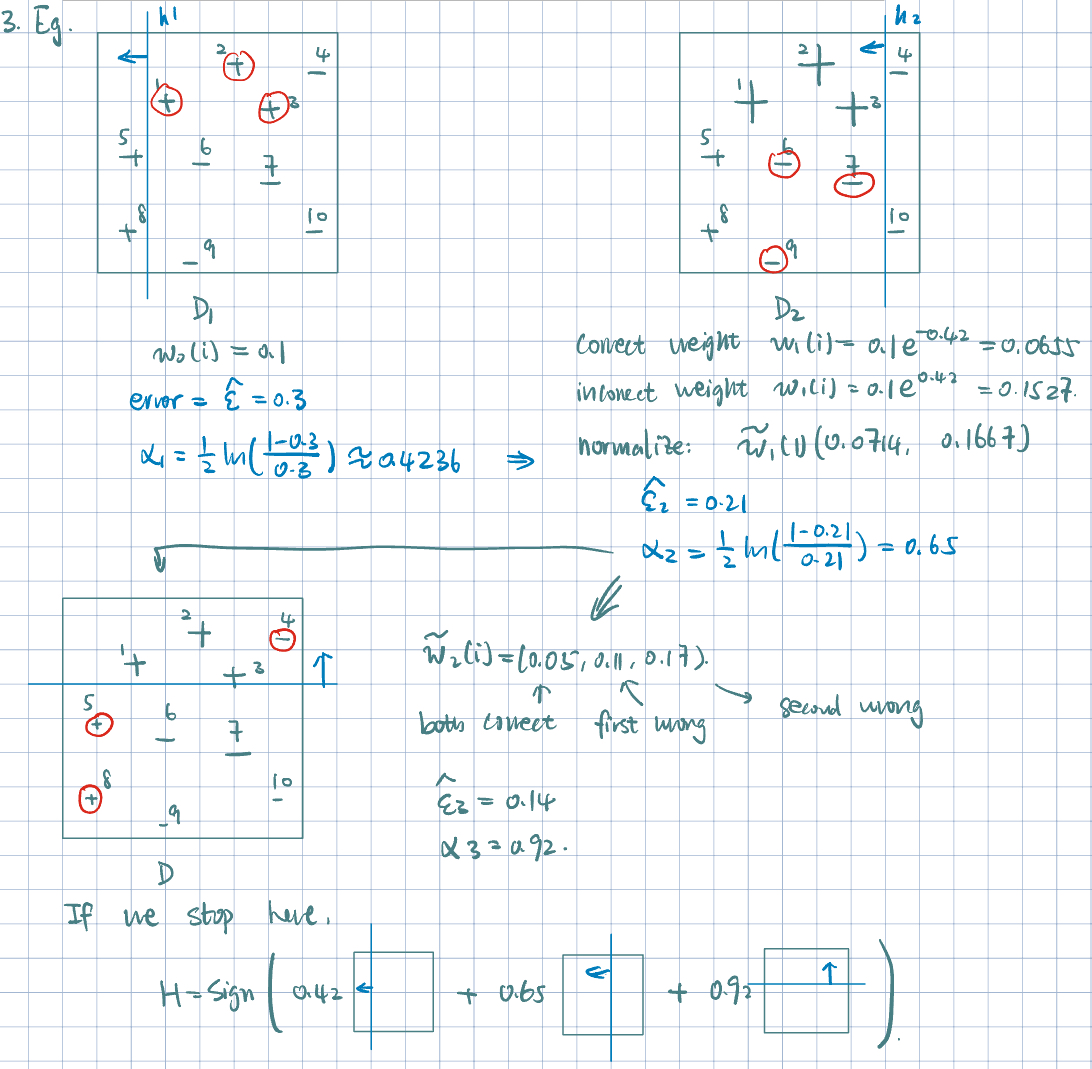
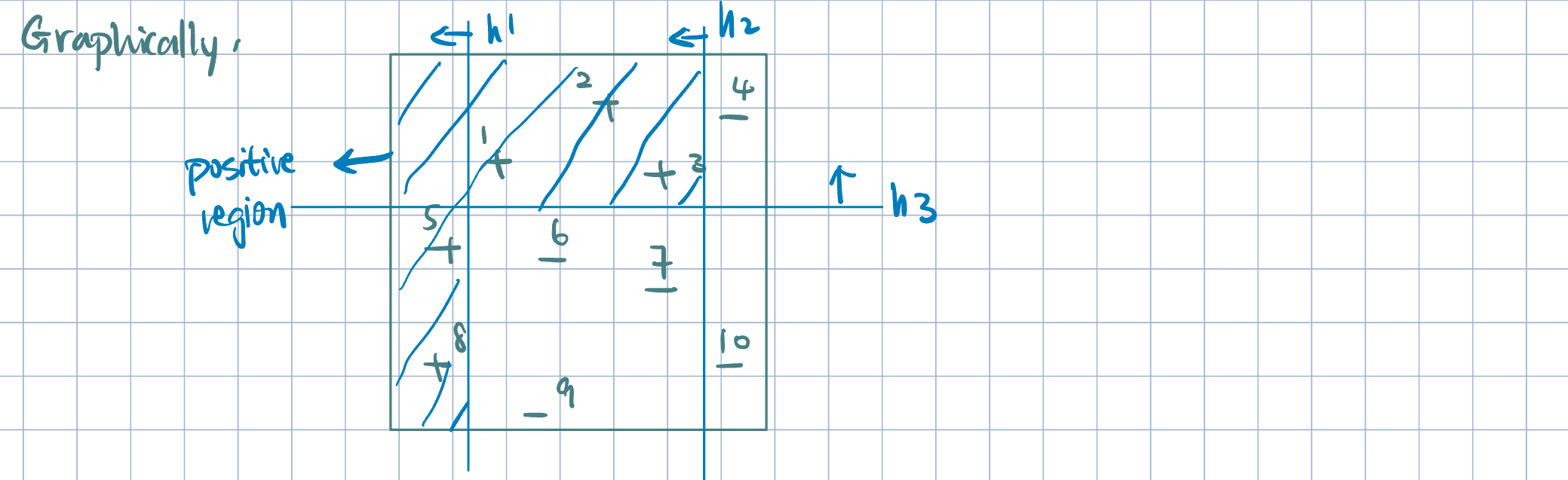
- Properties of Boosting:
- Weighted training error \(\hat\epsilon_m\) (for each iteration’s new weak error): tends to increase with each boosting iteration.
- Ensemble training error does not necessarily decrease monotonically. Ensemble exponential loss decreases monotonically (as this is what we are minimizing).
- Ensemble test error (generalization error) does not increase even after a large number of boosting iterations (more robust to overfitting).