8 Decision Trees and Random Forest

This lecture discusses the basics od decision trees including how to build a decision tree. It also introduces ensemble methods and discusses the random forest algorithm as an example of ensemble methods.

Decision Tree

• Interpretability: Given a linear classifier dinfed by \(\va\theta=[\theta_1,\theta_2,\dots,\theta_d]\). How can we interpret the meaning of each parameter/coefficient? \[\norm{\theta_i}\text{: how this feature contributes to the decision.}\] To fit nonlinear model, we can use kernels. However, with kernels, the fitted parameter \(\va\theta\) becomes a blackbox, and we lose interpretability (especially when we use RBF kernels, \(\va\theta\in\R^\infty\)).
• A different approach: Decision Tree \[f:\mathcal{X}\to\mathcal{Y}\]
  • Both features (\(\mathcal{X}\)) and labels (\(\mathcal{Y}\)) can be a continuous, descrete, or binary value.

Example 1 (Forming a Decision Tree) Suppose \(\va x\in\qty{0,1}^2\)

\(x_1\)	\(x_2\)	\(y\)
1	1	0
1	0	1
0	1	1
0	0	0

Figure 1: Decision Tree

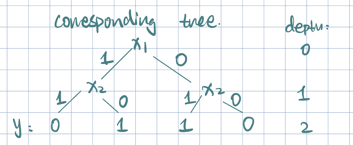
• We can use a boolean function of input feature to represent a decision tree.

Remark 1.

• As the number of nodes increases, the hypothesis space grows.
• Trivial solution: each examples has its own leaf node. If \(\va x\in\qty{0,1}^d\), then we have \(2^d\) leaf nodes.
• Problem: overffing, unlikely to generalize to unseen examples.

• Goal: Find the smallest tree that performs well on training data.
  • However, finding the optimal partition of the data is NP-complete (hard).
  • Instead, we can use a greedy appraoch:
    • Start with empty tree.
    • Find best feature to split on.
    • Recursively build branches into subtree.

Entropy, Conditional Entropy, and Information Gain

Example 2 (How to Find the Best Split) We want to predict whether ot not a flight will get delayed: \[\text{training data: }\begin{cases}29\text{ positive}\\35\text{ negative}\end{cases}\implies[29^+, 35^-].\] Suppose \(\va x=[x_1,x_2]\) are two binary features:

Figure 2: First Slipt

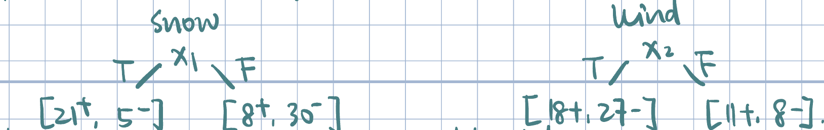
Splitting by snow is better because it produces more certain labels. But, how do we measure uncertainty?

Definition 1 (Shannon’s Entropy) Let \(D_N\) be the training data, \(y\in\qty{-1,+1}\) be the binary outcome/label.

• \(\P_\oplus\): fraction of positive examples

• \(\P_\ominus\): fraction of negative examples \[\text{Entropy of }D_N=-\qty\Big(\P_\oplus\log_2\P_\oplus+\P_\ominus\log_2\P_\ominus)\]

• The definition uses \(\log_2\) because entropy is measured in bits.

• It measures the expected number of bits needed to encode a randomly drawn value of \(y\).

Figure 3: Plot of Entropy

• More generally, for categorical outcome \(y\in\qty{y_1,y_2,\dots,y_k}\), \[ \begin{aligned} H(y)&=-\qty\Big(\P(Y=y_1)\log_2\P(Y=y_1)+\P(Y=y_2)\log_2\P(Y=y_2)+\cdots+\P(Y=y_k)\log_2\P(Y=y_k))\\ &=-\sum_{i=1}^k\P(Y=y_i)\log_2\P(Y=y_i) \end{aligned} \]

• Note: entropy is usually positive as \(\log_2\P(Y=y_i)\) is negative.

• Entropy and Peakyness:
  • Imagine rolling a die and plotting the empirical distribution:
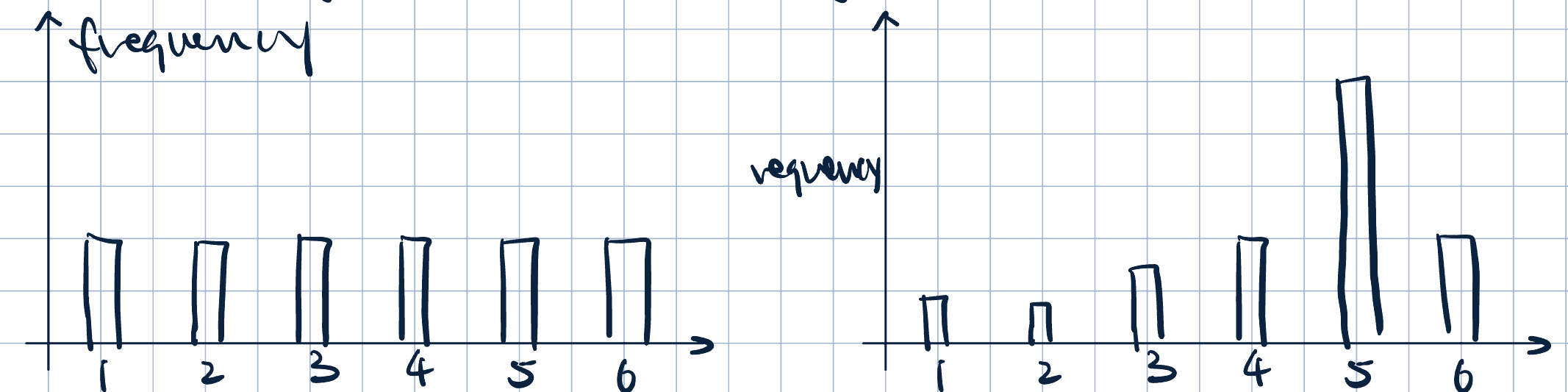
    • On the left: high entropy, more uncertain about the label, less peaky distribution
    • On the right: low entropy, less uncertain about the label, more peaky distribution

Definition 2 (Conditional Entropy) \[H(Y\mid X=x)=-\qty(\sum_{i=1}^k\P(Y=y_i\mid X=x)\log_2\P(Y=y_i\mid X=x))\] \[H(Y\mid X)=\sum_{x\in X}\P(X=x)\cdot H(Y\mid X=x)\]

• \(H(Y\mid X)\) shows the average surprise of \(Y\) when \(X\) is known.

Remark 2.

• When does \(H(Y\mid X)=0\)? When \(Y\) is completely determined by \(X\).
• When does \(H(Y\mid X)=H(Y)\)? When \(Y\independ X\).
• We can use conditional entropy to measure the quality of a split:
  • Idea: if knowing \(x_1\) reduces uncertainty more than knowing \(x_2\), we should split by \(x_1\).

Definition 3 (Information Gain (IG) / Mutual Information) \[ IG(X;Y)=H(Y)-H(Y\mid X), \]

• where \(H(Y)\) is the entropy of parent node, and \(H(Y\mid X)\) is the average entropy of the children note.
• \(IG\) measures the amount of information we learn about \(Y\) by knowing the value of \(C\) (and vice versa \(\implies\) symmetric).

Example 3 (Back to the Example) We want to predict whether ot not a flight will get delayed: \[\text{training data: }\begin{cases}29\text{ positive}\\35\text{ negative}\end{cases}\implies[29^+, 35^-].\] Suppose \(\va x=[x_1,x_2]\) are two binary features:

Figure 4: First Slipt

• Calculate entropy of \(y\): \[H(y)=-\qty(\dfrac{29}{64}\log_2\dfrac{29}{64}+\dfrac{35}{64}\log_2\dfrac{35}{64})\approx0.9937\]

• Calcualte the conditional entropy for each feature: \[ \begin{aligned} H(y\mid x_1)&=\dfrac{26}{64}\qty(-\dfrac{21}{26}\log_2\dfrac{21}{26}-\dfrac{5}{26}\log_2\dfrac{5}{26})+\dfrac{38}{64}\qty(-\dfrac{8}{38}\log_2\dfrac{8}{38}-\dfrac{30}{38}\log_2\dfrac{30}{38})\\ &=0.7278\\\\ H(y\mid x_2)&=\dfrac{45}{64}\qty(-\dfrac{18}{45}\log_2\dfrac{18}{45}-\dfrac{27}{45}\log_2\dfrac{27}{45})+\dfrac{19}{64}\qty(-\dfrac{11}{19}\log_2\dfrac{11}{19}-\dfrac{8}{19}\log_2\dfrac{8}{19})\\ &=0.9742. \end{aligned} \]

• Calcualte the information gain: \[ \begin{aligned} IG(x_1;y)&=0.9937-0.7278=0.2659\\ IG(x_2;y)&=0.9937-0.9742=0.0195. \end{aligned} \] So, \(IG(x_1;y)>IG(x_2;y)\), \(x_1\) is a better split.

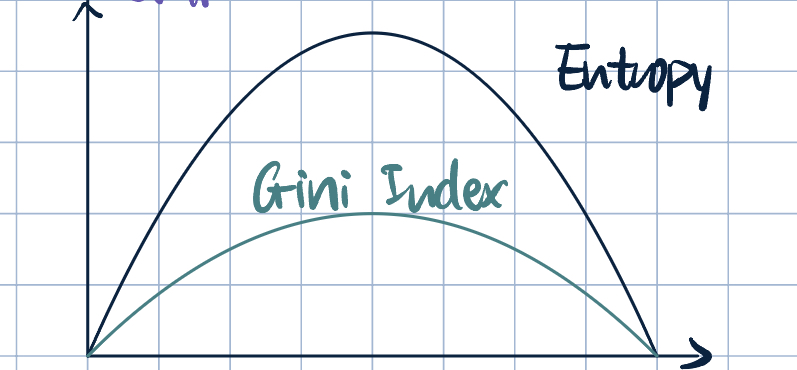
• Another Measure of Uncertainty: Gini Index and Gini Gain: \[ \begin{aligned} \text{Gini}(Y)&=\sum_{k=1}^k\P(Y=y_k)\qty(1-\P(Y=y_k))=1-\sum_{k=1}^k\P(Y=y_k)^2\\ \text{GiniGain}(X;Y)&=\text{Gini}(Y)-\sum_{x\in X}\P(X=x)\text{Gini}(Y\mid X=x). \end{aligned} \]

Remark 3. In practice, using \(IG\) or \(\text{GiniGain}\) may lead to different results, but it is unclear how different it can be.

Figure 5: Gini Index and Entropy Plot

Learning Decision Trees: A Greedy Approach

\[ \begin{aligned} \arg\max_{j=1,\dots,d}IG(x_j;y)&=\arg\max_j H(y)-H(y\mid x_j)\\ &=\arg\min_j H(y\mid x_j). \end{aligned} \]

• When to stop growing a tree? (Stopping Criteria)
  • When all record have the same label (assume no noise).
  • If all record have identical features (no further splits possible).

Remark 4. We should not stop when all stributtes have \(0\ IG\). See Example 1.

\begin{algorithm} \caption{Building Decision Tree} \begin{algorithmic} \Procedure{BuildTree}{$DS$} \IF{$y^{(i)}==y$ for all examples in $DS$} \Return{$y$} \ElseIf{$x^{(i)}==x$ for all examples in $DS$} \Return{majority label} \Else \State $x_s=\argmin_x H(y\mid x)$ \For{each value $v$ of $x_s$} \State $DS_y=\qty{\text{examples in }DS\text{ where }x_s=v}$ \State BuildTree($DS_y$)$\qquad$\Comment{recursive function} \EndFor \EndIf \EndProcedure \end{algorithmic} \end{algorithm}

• How do we avoid overfitting? We want simpler trees.
  • Set a maximum depth
  • Measure performance on validation data. If growing tree results in worse performance, stop.
  • Post-prune: grow entire/full tree and then greedily remove nodes that affect validation error the least.

Ensemble Methods and Random Forest

• Goal: Descreae variance without increasing bias (recall bias-variance trade-off)
• Idea: Average across multiple models to reduce estimation error. But we only have one single training set, how can we learn multiple models? BAGGING

Bootstrap Aggregatting (BAGGING)

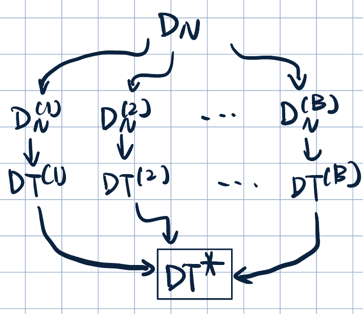
• General procedure:
  • Create \(B\) bootstrap samples: \(D_N^{(1)},\dots,D_N^{(B)}\)
  • Train decision tree on each \(D_N^{(b)}\)
  • Classify new examples by majority vote (i.e., mode)

Figure 6: BAGGING

• Why does bagging work? (Assume \(y\in\qty{-1,+1}\))
  • Suppose we have \(B\) independent classifers: \[\hat f^{(b)}:\R^d\to\qty{-1,+1},\] and each \(\hat f^{(b)}\) has a misclassification rate of \(0.4\).
    • That is, if \(y^{(i)}=+1\), then \(\P\qty(\hat f^{(b)}(\va x^{(i)})=-1)=0.4\quad\forall b=1,\dots,B\) and \(\forall\ i,\dots,d\)
  • Now, applay baaged classifier: \[\hat f^{(\text{bag})}(\va x)=\arg\max_{y\in\qty{-1,+1}}\sum_{b=1}^B\1\qty(\hat f^{(b)}(\va x)=\hat y)=\arg\max\qty{B_{-1},B_{+1}},\] where \(B_{-1}\) is the number of votes for \(-1\), and \(B_{+1}\) is the number of votes for \(+1\). Then, \[B_{-1}\sim\text{Binomial}(B,0.4).\] Recall: if \(X\sim\text{Binomial}(n,p)\), then the probability of getting exactkly \(k\) successes in \(n\) trails is given by \[P(X=k)=\binom{n}{k}p^k(1-p)^{n-k}.\] Thus, misclassification rate of bagged classifer is \[\begin{aligned}\P\qty(\hat f^{(\text{bag})}(\va x^{(i)})=-1)&=\P\qty(B_{-1}\geq\dfrac{B}{2})\\&=1-\P\qty(B_{-1}<\dfrac{B}{2})\\&=1-\sum_{k=1}^{\lfloor B/2\rfloor}\binom{B}{k}(0.4)^k(1-0.4)^{B-k}.\end{aligned}\] Note: \[\lim_{B\to+\infty}\sum_{k=1}^{\lfloor B/2\rfloor}\binom{B}{k}p^k(1-p)^{B-k}=1\] as long as misclassification rate \(p<0.5\). So, as \(B\to\infty\), misclassification \(\to0\).
• Reality: Predcition error rarely goes to \(0\).
  • Bagging only reduces estimation error (varaince).
  • We don’t ahve independence assumption: classifiers trained on bootstrapped dataset are NOT independent.

Remark 5.

• On average, each bootstrap contain \(63.2\%\) of original data.
• How similar are boostrap samples?
  • Probability of example \((i)\) is not selected once: \(1-\dfrac{1}{n}\).
  • Probability of example \((i)\) is not selected at all: \(\qty(1-\dfrac{1}{n})^n\).
• Then, \[\lim_{n\to\infty}\qty(1-\dfrac{1}{n})^n=\dfrac{1}{e}\approx36.8\%.\] So, when \(n\to\infty\), the probability of example \((i)\) is not selected at all is \(36.8\%\).

Further Decorrelate Trees: Random Forest

• Random forest is an ensemble method designed specifically for trees (bagging applies more boardly).
• Two sources of randomness:
  • Bagging
  • Random feature subsets:at erach node, best split chosen from subset of \(m\) features instead of all \(d\) features.

\begin{algorithm} \caption{Random Forest} \begin{algorithmic} \State{\# Bagging} \For{$b=1,\dots, B$} \State draw bootstrap sample $D_N^{(b)}$ of size $N$ from $D_N$ \State grow decision tree $DT^{(b)}$$\qquad$\Comment{See below code for growing $DT^{(b)}$} \EndFor \Return{ensemble $\qty{DT^{(1)}, \dots, DT^{(B)}}$} \State{\# Subprocedure for growing $DT^{(b)}$; random feature subset} \While{stopping criteria not met} \State Recursively repeat following steps for each node of tree: \State 1. select $m$ features at random from $d$ features \State 2. pick best feature to split on (using $IG$ or $\text{Gini}$) \State 3. split node into childre. \EndWhile \State{\# Another option to do Steps 1 and 2: } \State{1. compute $IG$ for all $d$ features} \State{2. randomly pick from top $m$} \end{algorithmic} \end{algorithm}