7 Feature Selection and Kernels

Feature Engineering

Feature Selection

Kernels

This lecture discusses the feature selection and kernel methods. We will cover feature engineering and selection methods, kernel methods, and kernel tricks.

Author

Jiuru Lyu

Published

February 18, 2025

Feature Engineering

Types of Variables:
- Numerical: Discrete / Continuous.
- Categorical
- Ordinal: categocial with order. E.g., Temperature: Low, Medium, High.
Discretization of Numerical Features (Quantization / Bining)
- Numerical $\to$ Categorical
  - E.g., age: $[18,25], (25, 45], (45, 65], (65, 85], >85$ or binary: $\leq 65, >65$
- Why? Allow a linear model to learn nonlinear relationships
Missing data:
- Depend on how missing they are:
  - Drop examples with missing values
  - Drop features with missing values
- Imputation approaches:
  - Univariate imputation
  - Multivariate imputation
  - Nearest neighbor imputation
  - Missing indicators
Time Series Data:
- Summary statistics:
  - mean, std
  - min, median, max, Q1, Q3
  - cumulative sum
  - count
  - count above/below threshold
- Trend:
  - linear slopes
  - piece-wise slopes
- Periodic trends: fast fourier transform

Feature Selection

Motivation:
- When having few examples, but a learge number of features ($d\gg N$), it becomes very easy to overfit the model.
- We need to remove uninformative features.
Methods:
- Filter method: before model fitting
- Wrapper method: after model fitting
- Embedded method: during model fitting
Filter Method: preprocessing*
- Rank individual features according to some statistical measure
- Filter out features that fall below a certain threshold
  - E.g., sample variance, Person’s correlation coerfficient between feature and label, Mutal information, $\chi^2$-statistic for categorical/ordinal features.
Wrapper Method: Search
- View feature selection as a model selection problem
- Which feature to use: hyperparameter
  - E.g,b Brute-force, exhausitve search: If we have $d$ features, there are $2^d-1$ possible combinations. Computatianlly infeasible.
  - Greedy search: Forward selection, backward elimination.
- Forward selection:
  
  \begin{algorithm} \caption{Forward Selection} \begin{algorithmic} \State initialize $F$ to the set of all features \State initialize $S$ to the empty set $\qquad$\Comment{Start with $0$ features} \For{$i=1:d-1$} \For{ each feature $f\in F$} \State frain model using $(S, f)$ \State evaluate model \EndFor \State Select best set $\qty{S, f^*}$. $S=S+F^*$, and $F=F-f^*$ \EndFor \end{algorithmic} \end{algorithm}
  - This algorithm has complexity $\sim\bigO(d^2)$.
- Backward elimination:
  
  \begin{algorithm} \caption{Forward elimination} \begin{algorithmic} \State initialize $F$ to the set of all features \For{$i=1:d-1$} \State $S=$ set of all subsets of $F$ of size $d-i$. $\qquad$\Comment{Start with $d$ features} \For{ each subset $s\in S$} \State train model using $s$ \State evaluate model \EndFor \State Select best subset $s^*$, and $F=s^*$ \EndFor \end{algorithmic} \end{algorithm}
  - This algorithm has complexity $\sim\bigO(d^2)$. However, forward selection is less computationally expensive because we train more smaller modedls.
Embedded Method: Regularization
- Incorporate feature selection as part of the model fitting process
- Use $L_1$ (LASSO) regularization

	Filter	Wrapper	Embedded
Computational Cost	Fast. Only run once scalable to high dimension	Slow	Between filter and wrapper
Model/Algorithm Specific	Generic, agnostic to models and algorithms	Specific, considers model performance	Only applies to specific model / algorithms
Overfitting	Unlikely	Higher risk of overfitting	Regualrization controls overfitting

In practice, we use combinations of these methods.

Fitting Nonlinear Functions – Kernel Methods

Question: How can we use linear models to learn nonlinear trends?
- Map to higher order dimensions: e.g., $\mqty[1&x&x^2&\cdots&x^m]$
For example, classification:

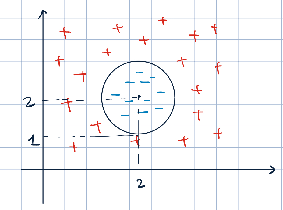
Figure 1: Higher Dimensional Classification
- Let $\va x=\mqty[x_1&x_2]^\top$ and $\phi(\va x)=\mqty[1&x_1&x_2&x_1x_2&x_1^2&x_2^2]^\top$.
- Find a linear classifier such that $\va\theta\cdot\phi(\va x)=0$ that perfectlly separates the two classes.
- Equation of a circle: $(x-h)^2+(y-k)^2=r^2$.
- In this example, $(x_1-2)+(x_2-2)^2=1$. So, $7-4x_1-4x_2+x_1^2+x_2^2=0$.
- Therfore, $\phi(\va x)=\mqty[1&x_1&x_2&x_1x_2&x_1^2&x_2^2]^\top$ and $\va\theta=\mqty[7&-4&-4&0&1&1]^\top$.
- But, we don’t want to use this method. Why?
  - Because dimension will blow-up. Suppose $\va x\in\R^d$ and $\phi(\va x)\in\R^p$. Then, \[p=\text{number of first and second order terms}=(d+1)+\dfrac{d(d+1)}{2}\sim\bigO(d^2).\]
  - We have $p\gg d$. It’s also likely that $p\gg N$.
  - In perceptron algorithm, our update complexity will then be $\sim\bigO(p)=\bigO(d^2)$, which is inefficient.
Key Observation:
- If we initialize $\va\theta^{(k)}=\va 0$, then $\va\theta^{(k)}$ is always in the span of feature vectors and can be expressed to linear combination of feature vectors: \[\va\theta^{(k)}=\sum_{i=1}^N\alpha_i\va x^{(i)}\quad\text{for some }\alpha_1,\alpha_2,\dots,\alpha_N.\]
- Then, we can rewrite the classifier to get \[\begin{aligned}h(\va x;\va\theta)&=\operatorname{sign}(\va\theta\cdot\va x)\\&=\operatorname{sign}\qty(\qty(\sum_{i=1}^N\alpha_i\va x^{(i)})\cdot\va x)\\&=\operatorname{sign}\qty(\sum_{i=1}^N\alpha_i\va x^{(i)}\cdot\va x).\end{aligned}\]
- Even if we are in higher dimensional feature space: \[h(\phi(\va x);\va\theta)=\operatorname{sign}\qty(\sum_{i=1}^N\alpha_i\qty(\phi(\va x^{(i)})\cdot\phi(\va x))).\]
- Classifiers now is written in $\alpha_i$ ($N$-dimensional) space, not in $\va x$ ($d$-dimensional) space.
- Then, the update rule is \[\alpha_i^{(k+1)}=\alpha_i^{(k)}+y^{(i)}.\]

\begin{algorithm} \caption{New Perceptron} \begin{algorithmic} \State $\va\alpha^{(0)}=\va 0\in\R^N$, $k=0$ \While{not converged} \For{$i=1,\dots,N$} \If{$y^{(i)}\qty(\sum_{j=1}^N\alpha_j\phi(\va x^{(i)})\cdot\phi(\va x^{(j)}))\leq 0$} \State $\alpha_{i}^{(k+1)}=\alpha_i^{(k)}+y^{(i)}$ \State $\alpha_j^{(k+1)}=\alpha_j^{(k)}$ when $j\neq i$ \State $k++$ \EndIf \EndFor \EndWhile \end{algorithmic} \end{algorithm}

$\phi(\va x^{(i)})\cdot\phi(\va x^{(j)})$ can be pre-computed. Complexity is $\bigO(N^2p)$
The update complexity $\bigO(1)$.
How can we speed up dot product $\phi(\va x)\cdot\phi(\va x')$? We can calculate the dot producrt $\phi(\va x)\cdot\phi(\va x')$ withtout calculating $\phi(\va x)$ and $\phi(\va x')$.

Example 1 Suppose $\phi(\va x)=\mqty[x_1^2&x_2^2&\sqrt{2}x_1x_2]^\top$. Then, \[ \begin{aligned} \phi(\va u)\cdot\phi(\va v)&=\mqty[u_1^2&u_2^2&\sqrt{2}u_1u_2]^\top\cdot\mqty[v_1^2&v_2^2&\sqrt{2}v_1v_2]^\top\\ &=u_1^2v_1^2+u_2v_2^2+2u_1u_2v_1v_2\\ &=(u_1v_1+u_2v_2)^2\\ &=\qty(\va u\cdot\va v)^2. \end{aligned} \]

Definition 1 (Kernel Function) Kernel function is an implicit feature mapping that allows us to compute the dot product in the feature space without explicitly computing the feature vectors. \[K:\underbrace{\R^d\times\R^d}_\text{feature vectors}\to\R\]

Theorem 1 (Common Kernels:)

Linear Kernel: \[K\qty(\va x^{(i)},\va x^{(j)})=\va x^{(i)}\cdot\va x^{(j)}.\]
Polynomial Kernel: \[K\qty(\va x^{(i)},\va x^{(j)})=\qty(\va x^{(i)}\cdot\va x^{(j)}+1)^d.\]
Radial Basis Function (RBF) Kernel: infinite-dimensional feature space \[\begin{aligned}K_\text{RBF}(\va u,\va v)&=\exp\qty(-\gamma\norm{\va u-\va v}^2)\\&=C\sum_{n=0}^\infty\dfrac{K_{\operatorname{poly}(n)}(\va u,\va v)}{n!}\end{aligned}\]

\begin{algorithm} \caption{Kernelized Perceptron} \begin{algorithmic} \State $\alpha_j^{(0)}=0$, $k=0$ \While{not converged} \For{$i=1,\dots,N$} \If{$y^{(i)}\qty(\sum_{j=1}^N\alpha_j^{(k)}K(\va x^{(j)}, \va x^{(i)}))\leq 0$} \State $\alpha_{i}^{(k+1)}=\alpha_i^{(k)}+y^{(i)}$ \State $\alpha_j^{(k+1)}=\alpha_j^{(k)}$ when $j\neq i$ \State $k++$ \EndIf \EndFor \EndWhile \end{algorithmic} \end{algorithm}