6 Model Selection and Model Assessment
Model Selection
Model Assessment
Classification Metrics
Regression Metrics
Cross Validation
This lecture discusses the model assessment and model selection process. We will cover classification performance metrics, regression metrics, model assessment process, and model selection.
Classification Performance
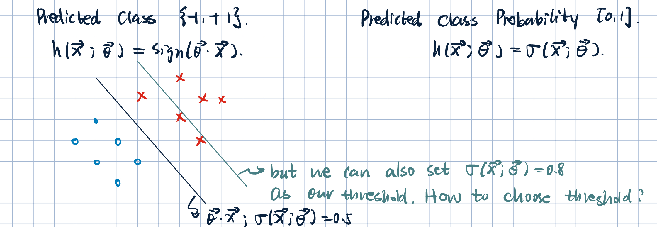
- Given \(\hat y=h(\va x;\va\theta)\) and \(D=\qty{\va x^{(i)}, y^{(i)}}_{i=1}^N\), \(\va x^{(i)}\in\R^d\) and \(y^{(i)}\in\qty{-1,+1}\).
- Misclassification error: \[\dfrac{1}{N}\sum_{i=1}^N\1[\hat y^{(i)}\neq y^{(i)}].\]
- Accuracy: \[\dfrac{1}{N}\sum_{i=1}^N\1[\hat y^{(i)}=y^{(i)}].\]
- What’s wrong with accuracy: It can be misleading when we have disproportional groups. E.g., rare disease.
- Confusion Matrix and Classification Metrics:
| Predicted (\(-\)) | Predicted (\(+\)) | |
|---|---|---|
| Actual (\(-\)) | True Negative (TN) | False Positive (FP) Type I Error |
| Actual (\(+\)) | False Negative (FN) Type II Error | True Positive (TP) |
- Accuracy: \(\dfrac{TP+TN}{N}\)
- Sensitivity / True Positive Rate (TRR) / Recall: \(\dfrac{TP}{TP+FN}\).
- Specificity / True Negative Rate (TNR): \(\dfrac{TN}{TN+FP}\).
- False Positive Rate (FPR): \(\dfrac{FP}{TN+FP}=1-\text{specificity}\).
- Precision / Positive Predictive Value (PPV): \(\dfrac{TP}{TP+FP}\).
Remark 1. If we predict everything to be positive, \(TN=FB=0\). Then, - Accuracy: \(\dfrac{TP}{N}\). - Sensitivity: \(1\). - Specificity: \(0\). - False Positive Rate: \(1\). - Precision: \(\dfrac{TP}{N}\).
- Composite Metrics: Trade-offs:
- Balanced Accuracy: mean of sensitivity and specificity. \[\dfrac{1}{2}\qty(\dfrac{TP}{TP+FN}+\dfrac{TN}{TN+FP})\]
- F1 Score: harmonic mean of precision and recall \[2\dfrac{\cdot\text{Precision}\cdot\text{Recall}}{\text{Precision}+\text{Recall}}\]
- Discrimination Thresholds:
- Receiver Operating Characteristic (ROC) Curve: TPR vs. FPR.
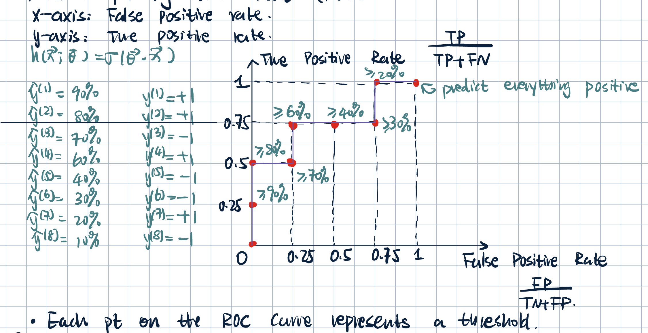
- Each point on the ROC curve corresponds to a threshold / a decision boundary.
- Each point represents a differenet trade-off between FPR and TPR.
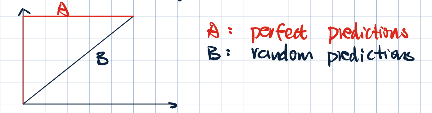
- Properties of ROC:
- Slope is always upward.
- Two non-intersecting curves means one model dominate the other.
- Perfect prediction vs. random prediction
- ROC shows the trade-off between sensitivity and specificity.
- but still not a very good summary metric: it is not a single number.
- Aread under the ROC Curve (AUROC, ROC-AUC):
- Calculated using the trapezoid rule:
sklearn.metrics.auc(x, y). - Intuitive meaning: Given two randomly chosen examples, one positive and one negative, the probability of ranking positive example higher than the negative example.
- \(AUC=1\) for perfect prediction, \(0.5\) for random prediction.
- \(AUC>0.9\): excellent prediction, but consider information leakage.
- \(AUC\approx0.8\): good prediction.
- \(AUC<0.5\): something is rong.
- Calculated using the trapezoid rule:
- Precision-Recall Curve and AUPRC:
- A high AUPRC represents both higher recall and precision.
- ROC curves should be used when there are rounghly equal numbers of observations for each class.
- Precision-Recall curves may be used when there is a moderate to large class imbalance.
- Receiver Operating Characteristic (ROC) Curve: TPR vs. FPR.
- Classifier Probability Calibration:
- When a model produce a probability of positive class, is that number actually a meaningful probability?
- For example, if my model predicts 90% for a set of examples, does that mean 90% of those examples ahve label \(+1\)?
- Multiple classes metrics:
- Accuracy: \[ACC=\dfrac{TP1+TP2+TP3+\cdots}{Total}\]
- Macro-average precision: \[PRE_\text{macro}=\dfrac{PRE_1+PRE_2+\cdots+PRE_n}{n}\]
- Micro-average precision (should not use): \[PRE_\text{micro}=\dfrac{TP1+TP2+TP3+\cdots}{TP1+TP2+TP3+\cdots+FP1+FP2+FP3+\cdots}\]
Regression Metrics
Given \(\hat y=f(\va x;\va\theta)\) and \(D=\qty{\va x^{(i)}, y^{(i)}}_{i=1}^N\), \(x^{(i)}\in\R^d\) and \(y^{(i)}\in\R\).
- Mean Squared Error (MSE): \[MSE=\dfrac{1}{N}\sum_{i=1}^N\qty(\hat y^{(i)}-y^{(i)})^2\]
- Root Mean Squared Error (RMSE): \[RMSE=\sqrt{MSE}=\sqrt{\dfrac{1}{N}\sum_{i=1}^N\qty(\hat y^{(i)}-y^{(i)})^2}\]
- Mean Absolute Error (MAE): \[MAE=\dfrac{1}{N}\sum_{i=1}^N\abs{\hat y^{(i)}-y^{(i)}}\]
- Mean Bias Error (MBE): \[MBE=\dfrac{1}{N}\sum_{i=1}^N\qty(y^{(i)}-y^(i))\]
Model Assessment Process
- Houldout: forming a test set:
- Hold out some data (i.e., test data) that are not used for training the modedl.
- Proxy for “everything you might see.”
- Procedure:
- On training data, we train our
model. - On test data, we use the
modelto makepredictions. - We compare the
predictionswith thetrue labelsto get theperformance.
- On training data, we train our
- Problem of holdout:
- Too few data for traiing: unable to properly learn from the data
- Too few for testing: bad approximation of the true error
- Rule of thumb: enough test samples to form a reasonable estimate.
- Common split size is \(70\%-30\%\) or \(80\%-20\%\).
- Question: what to do if we don’t have enough data? \(K\)-Fold Cross Validation (CV):
- Use all the data to train / test (but don’t use all data to train at the same time).
- Procesudre:
- Split the data into \(K\) parts or “folds.”
- Train on all but the \(k\)-th part and test / validate on the \(k\)-th part.
- Repeat for each \(k=1,2,\ldots,K\).
- Report average performance over \(K\) experiments.
- Common values of \(K\):
- \(K=2\): two-fold cross validation.
- \(K=5\) or \(K=10\): 5-fold or 10-fold cross validation – common choices.
- \(K=N\): leave-one-out cross validation (LOOCV).
- The choice of \(K\) is based on how much data we have.
- Monte-Carlo Cross Validation:
- AKA repeated random sub-sampling validation.
- Procedure:
- Randomly select (without replacement) some fraction of the data to form training set.
- Assign rest to test set.
- Repeat multiple times with different partitions.
| Method | How many possible partitions do we see? | How many models do we need to train? | What is the final model? | How to get error estimates? |
|---|---|---|---|---|
| Holdout | \(1\) | \(1\) | The model | Bootstrapping |
| \(K\)-Fold CV | \(K\) | \(K\) | Average of \(K\) models | Average of \(K\) error estimates |
| Monte-Carlo CV | as many as possible | as many as possible | Average of all models | Average of all error estimates |
- Bootstrapping to find Confidence Intervals:
- Sample with replacement \(N\) times.
- Calculate performance metric on each boostrap iterate.
- The 95% confidence interval is the \(2.5\)-th and \(97.5\)-th percentile of the boostrap distribution.
Model Selection
Goal: selecting the proper level of flexibility for a model (e.g., regularization strength in logistic regression)
- Select hyperparameters of the model: “meta-optimization”
- Regularization strength
- Regularization type
- Loss function
- Polynomial degree
- Kernal type
- Different from model parameters:
- Feature coefficients
- Simple, popular solution: \(K\)-fold CV for Hyperparameter Selection
- Assessment + Selection Guidelines:
- Do not use same samples to choose optimal hyperparameters and to estimate test / generalization error.
- Choice of methodology will depend on your problem and dataset.
- Three-way split:
- Training set: to train the model
- Validation set: to select hyperparameters
- Test set: to estimate generalization error
- Holdout + \(K\)-Fold CV:
- Holdout: test dataset to assess the performance.
- Training set: use \(K\)-fold CV to find optimal hyperparameters.
- Use optimal hyperparameters to train on the training data and assess on test.
- Nested CV:
- Outer \(K\)-fold loop: assess the performance.
- Inner \(K\)-fold loop: choose the optimal hyperparameters.
Tip 1: An Example in
sklearn
Most commonly used function/classes: train_test_split, KFold, and StratifiedKFold.
# generate an 80-10-10 train-validation-test three-way split
from sklearn.model_selection import train_test_split

X_train, X_test, y_train, y_test = train_test_split(X, y, test_size=0.1)
X_test, X_val, y_test, y_val = train_test_split(X_train, y_train, test_size=1/9)

# generate a 4-fold CV in a for-loop
# stratified k-foldL maintains label proportions
from sklearn.model_selection import StratifiedKFold

skf = StratifiedKFold(n_splits=5)
for train_idx, test_idx in skf.split(X, y):
    X_train, X_test = X[train_idx], X[test_idx]
y_train, y_test = y[train_idx], y[test_idx]- Hyperparameter Search Space:
- Grid Search CV: exhaustive search for the best hyperparameter values using cross validation.
sklearn.model_selection.GridSearchCV. - Randomized Search CV: random search over hyperparameters.
sklearn.model_selection.RandomizedSearchCV.
- Grid Search CV: exhaustive search for the best hyperparameter values using cross validation.