4 Regularization

This lecture starts from the bias-variance tradeoff, and then introduces regularization as a way to control the tradeoff. We will discuss the \(L_2\) regularization (Ridge Regression), \(L_1\) regularization (Lasso Regression), and Elastic Net.

Introduction: Bias-Variance Tradeoff

• Polynomial regression:
  • Instead of only using \(\phi(x)=[1,x]^\top\) , we can add higher dimension terms of feature: \[\phi(x)=[1,x,x^2,x^3,\dots]^\top\]
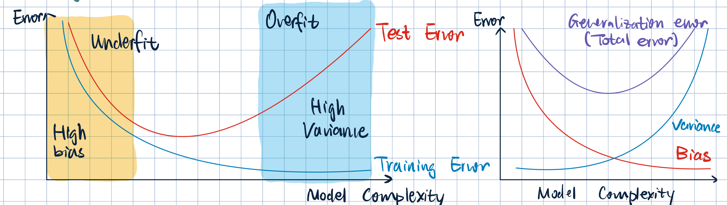
  • However, if we get too far, we will encounter overfitting.
• Overfitting and Underfitting:
  • If we optimize \(R(\va\theta, D)\), \(R(\va\theta, D_\text{test})\) can be learge due to:

Underfitting	Overfitting
Bias	Variance
Approximation error	Estimation error
Poor on training set	Good on training set
Poor on test set	Poor on test set
Adding more data will not help	Adding more data will help

Figure 1: Model Complexity vs. Error: Bias-Variance Tradeoff

• Sources of Bias:
  • Model class too small: unable to represent the underlying relationship
  • Models are “too global” (e.g., constant output, single linear separator)
• Reduing Bias: Use more complex models
  • Interaction terms
  • Add more features
  • Kernels
  • Algorithm-specific approaches
• Sources of Variance:
  • Noise in labels or features
  • Models are too “local” – sensitive to small changes in feature values
  • Training dataset too small.
• Reducing Variance: Collect more data, or less complex models
  • Drop interaction terms
  • Regualrization
  • Feature selection
  • Don’t use kernels
  • Ensemble
• Balancing Bias and Variance: Generalizable Model
  • But how to control the tradeoff? Regularization.

Regularization

Definition 1 (Regularization Training Error) A “knob” for controlling model complexity: \[ J(\va\theta)=\underbrace{R_N(\va\theta)}_\text{emiprical risk}+\underbrace{\lambda\Omega(\va\theta)}_\text{regularization term}, \] where \(\lambda\) is the regularization strength, \(\lambda>0\), and \(\Omega(\va\theta)\) is the regularizer/regularization penalty.

The regularization strength \(\lambda\) balances: - How well we fit the data, and - Complexity of model.

Then, our goal is to \(\displaystyle\min_{\va\theta}J(\va\theta)\).

• Common Regularizer:
  • \(L_2\): Ridge Regression \[\Omega(\va\theta)=\dfrac{\|\va\theta\|_2^2}{2}=\dfrac{1}{2}\sum_{j=1}^d\theta_j^2\]
  • \(L_1\): Lasso Regression \[\Omega(\va\theta)=\|\va\theta\|_1=\sum_{j=1}^d\abs{\theta_j}\]
  • Elastic net: \[\Omega(\va\theta)=\lambda_2\|\va\theta\|_2^2+\lambda_1\|\va\theta\|_1\]
• Effect of Regularization:
  • When minimizing \(J(\va\theta)\), we are still trying to minimize \(R_N(\va\theta)\), but at the same time, minimize \(\Omega(\va\theta)\)
    • Push parameters to small values
    • Resist setting parameters away from default of \(0\) unless data strong suggest otherwise.
  • Why are small values in \(\va\theta\) good?
    • Limit effect of small perturbations in individual factors on putput.
    • If \(\theta_j=0\) exactly, then \(j\)-th parameter is effective unused \(\implies\) feature selection.
    • Occam’s Razor (\(13\)-th century philosopher, William of Ockham): “When you have two competing hypotheses, the simpler one is preferred.”
• Ridge Regression (\(L_2\)-Regularized Linear Regression) \[J(\va\theta)=\sum_{i=1}^N\dfrac{(y^{(i)}-\va\theta\cdot\va x^{(i)})^2}{2}+\lambda\dfrac{\|\va\theta\|_2^2}{2},\] where \(\dfrac{1}{N}\) is absorbed into \(\lambda\).
  • SGD: \[\grad_{\va\theta}\qty(\dfrac{\qty(y^{(i)}-\va\theta\cdot\va x^{(i)})^2}{2}+\lambda\dfrac{\|\va\theta\|_2^2}{2})\] gradient of squared \(L_2\) norm: \(\|\va\theta\|_2^2=\theta_1^2+\cdots+\theta_d^2=\va\theta\cdot\va\theta\). So, \[\pdv{\theta_j}\qty(\|\va\theta\|_2^2)=2\theta_j.\] Then, we have \[ \begin{aligned} \grad_{\va\theta}\qty(\|\va\theta\|_2^2)=\grad_{\va\theta}(\va\theta\cdot\va\theta)&=\mqty[\displaystyle\pdv{\theta_1}\qty(\|\va\theta\|_2^2),\dots,\pdv{\theta_d}\qty(\|\va\theta\|_2^2)]\\ &=\mqty[2\theta_1,2\theta_2,\dots,2\theta_d]\\ &=2\va\theta. \end{aligned} \] Therefore, \[ \grad_{\va\theta}\qty(\dfrac{\qty(y^{(i)}-\va\theta\cdot\va x^{(i)})^2}{2}+\lambda\dfrac{\|\va\theta\|_2^2}{2})=-\qty(y^{(i)}-\va\theta\cdot\va x^{(i)})\va x^{(i)}+\lambda\va\theta. \] Hence, the SGD update rule is \[ \begin{aligned} \va\theta^{(k+1)}=\va\theta^{(k)}-\eta_k\eval{\qty[-\qty(y^{(i)}-\va\theta\cdot\va x^{(i)})\va x^{(i)}+\lambda\va\theta]}_{\va\theta=\va\theta^{(k)}}\\ &=\va\theta^{(k)}+\eta_k\qty(y^{(i)}-\va\theta^{(k)}\cdot\va x^{(i)})\va x^{(i)}-\eta_k\lambda\va\theta^{(k)}\\ &=\underbrace{(1-\eta_k\lambda)}_{\text{between }0\text{ and }1}\va\theta^{(k)}+\underbrace{\eta_k\qty(y^{(i)}-\va\theta^{(k)}\cdot\va x^{(i)})\va x^{(i)}}_\text{same as before}. \end{aligned} \] The term \(1-\eta_k\lambda\) shrinks parameters towards \(0\) in each update.
  • Closed Form Solution: \[ \begin{aligned} J(\va\theta)&=\dfrac{1}{2}(X\va\theta-\va y)^\top(X\va\theta-\va y)+\dfrac{\lambda}{2}\va\theta^\top\va\theta\\ \grad_{\va\theta} J(\va\theta)&=(XX)\va\theta-X^\top y+\lambda\va\theta\\ &=(XX+\lambda I_d)\va\theta-X^\top y=0\\ \va\theta^*&=(\underbrace{XX+\lambda I_d}_\text{always invertible})^{-1}X^\top y. \end{aligned} \]
• Geometric Interpretation of Regularization: \[ \va\theta^*=\argmin_{\va\theta}R_N(\va\theta)+\lambda\Omega(\va\theta) \iff \min_{\va\theta}R_N(\va\theta)\quad\text{s.t.}\quad\Omega(\va\theta)\leq B. \]
  • We can transfer a constrained optimization problem to an unconstrained one by adding a penalty term.
  • They are equivalent by the Lagrange multiplier.

Figure 2: Geometric Interpretation of Regularization

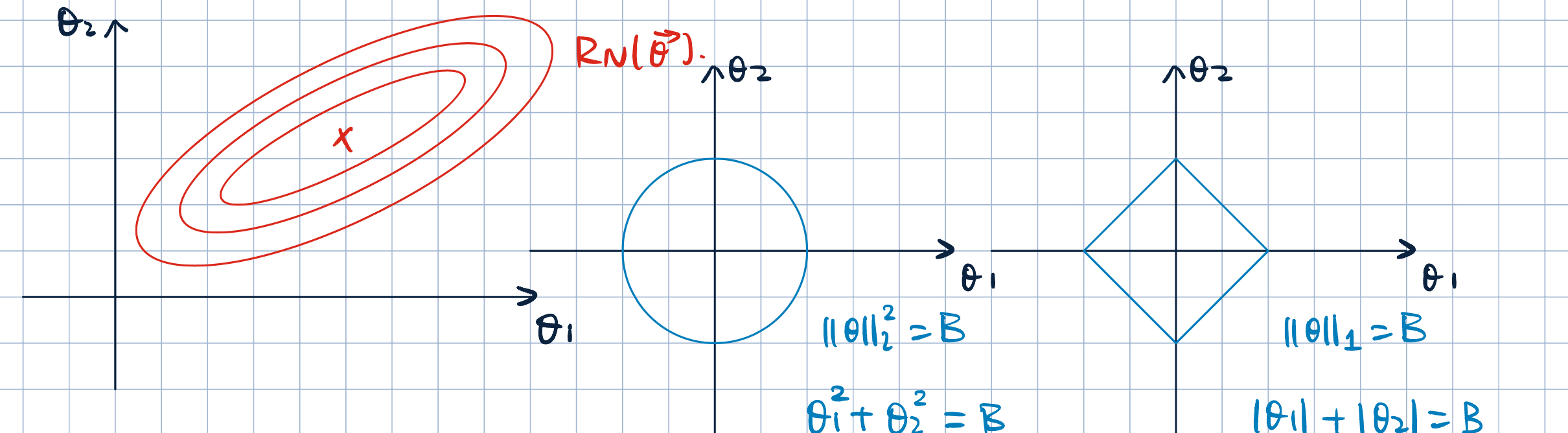
• Where is the optimal soltuion of the constrained optimization problem? The solution is the intersection of the level set of \(R_N(\va\theta)\) and the level set of \(\Omega(\va\theta)\).
• Method of Lagrange Multtiplier:
  • The pint where the level curve of function to minimize is tangent to (or just touching) the constraint.
• Intuition: two forces play
  • \(\Omega(\va\theta)\leq B\): shrink \(\va\theta\) towards winthin the constraint
  • \(\min R_N(\va\theta)\): move \(\va\theta\) towards the uncosntraied minimizer.
• \(L_2\) regularization will make parameters generally small.
• \(L_1\) regularization will make parameters sparse, and make some parameters exeactly \(0\).

Remark 1 (Remarks on Regularization).

• If there is an offset/intercept, this coefficient is usually left unpenalized (depending on the implementation).
  • If we write \(\va\theta\cdot\va x+b\) explicity, no penalty on \(b\).
  • If we write augmented parameters, then we penalize \(b\).
• Regularization can be “unfair” if features are on the different scales. So, we need feature pre-procesing (e.g., centering and normalization).
• Pratical usage of regression: sklearn

Function	Description
sklearn.linear_model.LinearRegression	closed form solution (wrapper of scipy.linalg.lstsq that uses SVD)
sklearn.linear_model.Ridge	Ridge regressionm, can select solver (SGD, SVD, etc.)
sklearn.linear_model.Lasso	Lasso regression, coordinate descent
sklearn.linear_model.ElasticNet	Elastic net, coordinate descent
sklearn.linear_model.SGDRegressor	generic SGD, mix and match different loss and regularizers

• Pratical use of linear classification: sklearn

Function	Description
sklearn.linear_model.LogisticRegression	logistic regression, can select solver (SGD, Newton-CG, etc.)
sklearn.linear_model.SGDClassifier	generic SGD, mix and match different loss and regularizers
sklearn.linear_model.Perceptron	perceptron, SGD with hinge loss
sklearn.svm.LinearSVC	linear SVM, hinge loss (support vector machine)
sklearn.svm.SVC	non-linear SVM, kernel trick