3 Linear Regression

This lecture discusses the linear regression, a fundamental concept in machine learning. It introduces the squared loss function and the update rule for gradient descent. It also derived the closed-form solution for linear regression using matrix notation.

Goal: Given data \(\qty{\va x^{(i)}, y^{(i)}}_{i=1}^N\), find a linear model \[ f(\va x;\va\theta)=\va\theta\cdot\va x, \] such that minimizes the empirical loss.

The Loss Function

Definition 1 (Squared Loss Function) The empirical loss for linear regression is defined by \[ R_N(\va\theta)=\dfrac{1}{N}\sum_{i=1}^N\operatorname{loss}\qty(y^{(i)}, \va\theta\cdot\va x^{(i)}), \] where loss is the squared loss: \[ \operatorname{loss}(z)=\dfrac{z^2}{2}. \]

This loss function is continuous, differentiable, and convex.

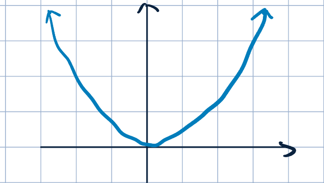
Here is a graph of the squared loss function:

Figure 1: Squared Loss

Intuition: we permits small discrepancies but penalizes large deviations.

Ordinary Least Squares (OLS)

• We will minimize the empirical loss with squared loss, i.e., \[ R_N(\va\theta)=\dfrac{1}{N}\sum_{i=1}^N\dfrac{\qty(y^{(i)}-\va\theta\cdot\va x^{(i)})^2}{2}, \] using SGD algorithm
• Recall the gradient descent update rule: \[ \va\theta^{(k+1)}=\va\theta^{(k)}-\eta_k\eval{\grad_{\va\theta}\operatorname{loss}(y^{(i)}\va\theta\cdot\va x^{(i)})}_{\va\theta=\va\theta^{(k)}} \]

In OLS case, we have \[ \begin{aligned} \grad_{\va\theta}\operatorname{loss}(y^{(i)}-\va\theta\cdot\va x^{(i)})&=\grad_{\va\theta}\dfrac{\qty(y^{(i)}-\va\theta\cdot\va x^{(i)})^2}{2}\\ &=-\qty(y^{(i)}-\va\theta\cdot\va x^{(i)})\va x^{(i)}. \end{aligned} \]

So, the update rule is \[ \va\theta^{(k+1)}=\va\theta^{(k)}+\eta_k\qty(y^{(i)}-\va\theta\cdot\va x^{(i)})\va x^{(i)}. \]

\begin{algorithm} \caption{SGD for Least Squares Regression} \begin{algorithmic} \State $k=0$; $\va\theta^{(0)}=\va 0$ \While{not converged} \State randomly shuffle points \For{$i=1,\dots, N$} \State $\va\theta^{(k+1)}=\va\theta^{(k)}+\eta_k\eval{\qty(y^{(i)}-\va\theta\cdot\va x^{(i)})\va x^{(i)}}_{\va\theta=\va\theta^{(k)}}$ \State $k++$ \EndFor \EndWhile \end{algorithmic} \end{algorithm}

Remark 1 (Compare with Hinge Loss Classification).

• We make updates on every data points
• Stopping criteria, learning rate, shuffling, etc., are the same.

Closed-Form Solution

• Since \(R_N(\va\theta)\) with squared loss is a covex function and differentiable everywhere, we can try to minimize it analytically by setting the gradient to \(0\).
• Rewrite empirical risk in matrix notation: \[ X=\mqty[-&\va x^{(1)\top}&-\\&\vdots&\\-&\va x^{(N)\top}&-]_{N\times d}\quad\text{and}\quad \va y=\mqty[y^{(1)}\\\vdots\\y^{(N)}]_{N\times 1}. \] Then, the empirical risk is \[ \begin{aligned} R_N(\va\theta)=\dfrac{1}{2}\dfrac{1}{N}\sum_{i=1}^N\qty(y^{(i)}-\va\theta\cdot\va x^{(i)})^2&=\dfrac{1}{2N}\qty(X\va\theta-\va y)^\top\qty(X\va\theta-\va y)\\ &=\dfrac{1}{2N}\qty(\va\theta^\top X^\top X\va\theta-2\va\theta^\top (X^\top\va y)+\va y^\top\va y). \end{aligned} \]

Tip 1: Commonly Used Differentiation Rules

\(f(\va x)\)	\(\grad_{\va x}f(\va x)\)
\(\va v^\top\va x\)	\(\va v\)
\(\va x^\top\va x\)	\(2\va x\)
\(\va x^\top A\va x\)	\((A+A^\top)\va x\) 1

• Therefore, the gradient of \(R_N(\va\theta)\) is

\[ \begin{aligned} \grad_{\va\theta}R_N(\va\theta)&=\dfrac{1}{2N}\qty(2X^\top X\va\theta-2(X^\top\va y))\\ &=\dfrac{1}{N}\qty(X^\top X\va\theta-X^\top\va y). \end{aligned} \]

• Set gradient to \(0\), we have

\[ \begin{aligned} \grad_{\va\theta}R_N(\va\theta)&=0\\ \dfrac{1}{N}\qty(X^\top X\va\theta-X^\top\va y)&=0\\ X^\top X\va\theta-X^\top\va y&=0\\ X^\top X\va\theta&=X^\top\va y\\ \va\theta^*&=\qty(X^\top X)^{-1}X^\top\va y. \end{aligned} \]

Remark 2 (Normal Equation and Inveritibility).

• The solutions is called the Normal Equation or the OLS solution.
• OLS solution \(\va\theta^*=\qty(X^\top X)^{-1}X^\top\va y.\) exists only when \(X^\top X\) is invertible.
• Invertibility of \(X^\top X\): “Gram matrix”
  • Why might it be non-invertible/singular/degenerate? \[\rank(X^\top X)\leq\rank(X)\leq\min\qty{N,d}\]
    • If \(d>N\), then \(\rank(X^\top X)\leq N<d\). Since \(X^\top X\in\R^{d\times d}\), we know \(X^\top X\) is not full rank, and thus non-invertible.
    • For example, if we have duplicated features, say \(x_1=x_2\), then if \(\mqty[\theta_1,\theta_2]\) is a solution, then \(\mqty[\theta_1-c,\theta_2+c]\) is also a solution.
  • What to do if \(X^\top X\) is not invertible?
    • Monro-Penrose Pseudo-Inverse: \[\va\theta^*=(X^\top X)^{\dagger}X^\top \va y=X^{\dagger}\va y\]
    • Regularization: See next lecture.

Footnotes

1. If \(A\) is symmetric, then \(\grad_{\va x}f(\va x)=2A\va x\).