2 Gradient Descent on Classification

This lecture discusses the gradient descent algorithm and its application to classification problem.It introduces the hinge loss function and the update rule for gradient descent.

Goal: Learning to classify non-linearly separable data (by considering a different objective function).

Objective Function and Hinge Loss

Definition 1 (Objective Function for Perceptron Algorithm) \[ \epsilon_{N}(\va\theta)=\sum_{i=1}^N\1\qty{-y^{(i)}(\va\theta\cdot\va x^{(i)})\leq0}, \] for conciseness, we assume the offset parameter is implicity. Note that the empirical risk is \[ R_N(\va\theta)=\frac{1}{N}\sum_{i=1}^N\operatorname{loss}\qty(y^{(i)}\qty(\va\theta\cdot\va x^{(i)})), \] so, training error is a special case of empirical risk.

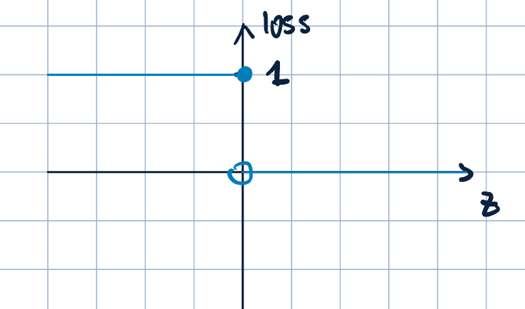
• Previously, we were using “zero-one loss”. Let \(z=y(\va\theta\cdot\va x)\), then the zero-one loss is \[ \operatorname{loss}_{0-1}(z)=\1\qty{z\leq0}=\begin{cases}1\quad&\text{if }z\leq 0\\0\quad&\text{o.w}\end{cases}. \]

The graph of the zero-one loss is shown below:

Figure 1: Zero One Loss

• However, there are some issues with the zero-one loss:
  • Not continuous at \(z=0\).
  • Not differentiable at \(z=0\).
  • Not convex.
• Due to these issues, direct minimization of empirical risk with \(0-1\) loss is chanllenging for the general case (NP-hard).

Tip 1: Calculus Refresher

• Continuous: A function \(f\) is continuous at \(x_0\) if \[\lim_{x\to x_0}f(x)=f(x_0)\].
• Differentiable: A function \(f\) is differentiable at \(x_0\) if the following limit exists: \[\lim_{h\to 0}\frac{f(x_0+h)-f(x_0)}{h}\] Also, Differentiable \(\implies\) continuous.
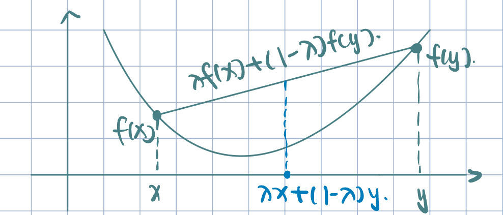
• Convex/concave up: \[f(\lambda x+(1-\lambda)y)\leq\lambda f(x)+(1-\lambda)f(y).\]

Figure 2: Convex Function

Example 1 (Motivation of Hinge Loss: Misclassification)  

Figure 3: Misclassification on Non-Linearly Separable Data

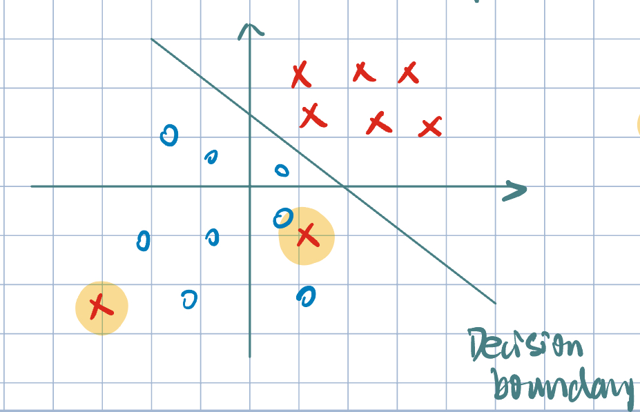
• Loss (or cost) associated with the ==misclassification== of these points is identified under \(0-1\) loss. Then, loss is \(1\) for each misclassified point.
• However, these two misclassifications are not equally bad.
• We need a loss function that treats these mistakes differently.

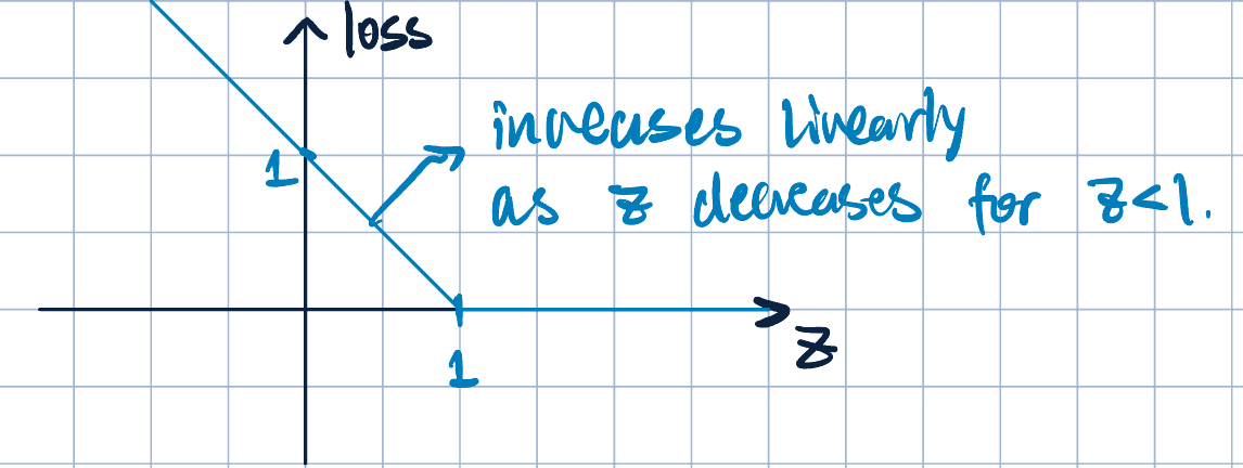
Definition 2 \[ \operatorname{loss}_h(z)=\max\qty{0,1-z}=\begin{cases}1-z\quad&\text{if }z\leq 1\\0\quad&\text{if }z>1\end{cases} \]

The graph of the hinge loss is shown below:

Figure 4: Hinge Loss

• Properties of hinge loss:
  • Non-negative.
  • If \(z=y\qty(\va\theta\cdot\va x)<1\), we incur a non-zero cost.
  • This forces predictions to be more than just correct, but we need \[y\qty(\va\theta\cdot\va x)\geq 1.\] Note, previously, we only imposed \(y\qty(\va\theta\cdot\va x)>0\).

Remark 1 (What does \(z=y\qty(\va\theta\cdot\va x)\) tell us?).

• Sign: correct (\(>0\)) or wrong (\(<0\)).
• Magnitude: how wrong (the larger, the more wrong). \[ \abs{y\qty(\va\theta\cdot\va x)}=\abs{y}\cdot\abs{\va\theta\cdot\va x}, \] where \(\abs{y}=1\) since \(y\in{-1,+1}\) and \(\dfrac{\abs{\va\theta\cdot\va x}}{\norm{\va\theta}}\) is the distance from the point to the decision boundary.

Definition 3 (Empirical Risk with Hinge Loss) \[ R_N(\va\theta)=\dfrac{1}{N}\sum_{i=1}^N\max\qty{0, 1-y^{(i)}\va\theta\cdot\va x^{(i)}} \] Why is it better/easier to minimize? - Continuous - (Sub)differentiable - Convex \(\implies\) We can use a simple algorithm to minimize it: Gradient Descent.

Gradient Descent

• Gradient:
  • Univariate case: \(f:\R\to\R\), \(y=f(x)\). Its derivative is \(f'(x)=\dsst\dv{x} f(x)\). \(f'(x)\) represents the rate of change:
    • \(f'(x)>0\): increasing
    • \(f'(x)=0\): a critical point
    • \(f'(x)<0\): decreasing.
  • Multivariate case: \(f:\R^d\to\R\), \(y=f(\va x)=f(x_1,x_2,\dots,x_d)\). Its gradient is \[\grad_{\va x} f(\va x)=\mqty[\dsst\pdv{x_1} f(\va x),\dots,\dsst\pdv{x_d} f(\va x)]^\top.\] The gradient points in the direction of the steepest ascent.
• Gradient Descent (GD):
  • Suppose we want to minimize some \(f(\va\theta)\) with respect to \(\va\theta\). We know gradient \(\grad_{\va\theta}f(\va\theta)\) points in the direction of steepest increase.
  • Idea: start somewhere, and take small steps in the opposite direction as gradient.

\begin{algorithm} \caption{Gradient Descent (GD)} \begin{algorithmic} \State $k=0$; $\va\theta^{(0)}=\va 0$ \While{not converged} \State $\va\theta^{(k+1)}=\va\theta^{(k)}-\underbrace{\eta_k}_{\substack{\text{learning}\\\text{rate}}}\overbrace{\eval{\grad_{\va\theta} f(\va\theta)}_{\va\theta=\va\theta^{(k)}}}^{\substack{\text{evaluate gradient}\\\text{at current }\va\theta}}$ \State $k++$ \EndWhile \end{algorithmic} \end{algorithm}

• Improve GD (Algorithm 1): Stochastic Gradient Descnet (SGD):
  • In GD (Algorithm 1), we need to compute the gradient over the entire dataset. This can be expensive for large datasets.
  • In SGD (Algorithm 2), we compute the gradient for each data point and update \(\va\theta\) accordingly.

\begin{algorithm} \caption{Stochastic Gradient Descent (SGD)} \begin{algorithmic} \State $k=0$; $\va\theta^{(0)}=\va 0$ \While{not converged} \State randomly shuffle points \For{$i=1,\dots, N$} \State $\va\theta^{(k+1)}=\va\theta^{(k)}-\eta_k\eval{\grad_{\va\theta}\operatorname{loss}(y^{(i)}\va\theta\cdot\va x^{(i)})}_{\va\theta=\va\theta^{(k)}}$ \State $k++$ \EndFor \EndWhile \end{algorithmic} \end{algorithm}

• Gradient for Hinge Loss: \[ \operatorname{loss}_h(z)=\max\qty{0,1-y\va\theta\cdot\va x} \]

\(\boxed{\text{Case I}}\) If \(y^{(i)}\va\theta\cdot\va x^{(i)}\geq 1\): loss is zero. Already at minimum. No update.

\(\boxed{\text{Case II}}\) If \(y^{(i)}\va\theta\cdot\va x^{(i)}<1\): loss is \[1-y^{(i)}\va\theta\cdot\va x^{(i)}\] Note that \(\va\theta\cdot\va x=\theta_1x_1+\theta_2x_2+\cdots+\theta_dx_d\), we have \[ \grad_{\va\theta}(\va\theta\cdot\va x)=\mqty[x_1,x_2,\dots,x_d]^\top=\va x. \] So, the gradient is \[ \begin{aligned} \grad_{\va\theta}\operatorname{loss}_h(y^{(i)}\va\theta\cdot\va x^{(i)})&=\grad_{\va\theta}(1-y^{(i)}\va\theta\cdot\va x)\\ &=0-y^{(i)}\grad_{\va\theta}(\va\theta\cdot\va x)\\ &=-y^{(i)}\va x^{(i)}. \end{aligned} \]

So, in Algorithm 2, the update rule is

\[ \begin{aligned} \va\theta^{(k+1)}&=\va\theta^{(k)}-\eta_k\eval{\grad_{\va\theta}\operatorname{loss}(y^{(i)}\va\theta\cdot\va x^{(i)})}_{\va\theta=\va\theta^{(k)}}\\ &=\va\theta^{(k)}+\eta_ky^{(i)}\va x^{(i)}. \end{aligned} \]

Remark 2 (Why shuffle points in SGD?).

• Remove the effect of any unintended/aritifical ordering in the dataset.
• Faster convergence

• Stopping criteria
  • Check if empirical risk stops decreasing.
  • Check if parameter vector stop changing.
  • Note: make \(\operatorname{loss}=0\) does not work here since the data is not perfectly linearly separable.
• Learning rate/Step size/\(\eta\):
  • Too small: slow convergence.
  • Too large: overshot & never converge
  • A hyperparameter that can (and should) be tuned.
  • May set \(\eta\) as a constant or a function of \(k\). For example, \[\eta_k=\dfrac{1}{k}.\]

Theorem 1 (GD (Algorithm 1) and SGD (Algorithm 2) Convergence Theorem)  

• With appropriate learning rate \(\eta\), if \(R_N(\va\theta)\) is convex, (S)GD will converge to the global minimum almost surely.
• SGD is a general algorithm that can be applied to non-convex functions as well, in which case it converges to a local minimum.

Definition 4 (Robbins-Monro Conditions) A good learning rate ensures convergence satisfying the Robbins-Monro conditions: \[ \sum_{k=1}^\infty\eta_k=\infty\quad\text{and}\quad\sum_{k=1}^\infty\eta_k^2<\infty. \]

Remark 3 (Differentiability of Loss Function). \(R_N(\va\theta)\) with hinge loss is not everywhere differentiable since it si piecewise linear. What do we do? - When differentiable, use gradient. - When sub-differentiable, choose any gradient around the kink.