1 Linear Classification

This lecture discusses the linear classification, a fundamental concept in machine learning. It introduces loss functions, training error, and the perceptron algorithm.

Machine Learning Terminology

• feature vector: \(\va x=\mqty[x_1&x_2&\cdots&x_d]^\top\in\R^d\). \(\R^d\) is called the feature space.
• label: \(y\in\qty{-1,+1}\), binary.
• training set of labeled examples: \[D=\qty{\va x^{(i)},y^{(i)}}_{i=1}^N\]
• classifier: \[h:\R^d\to\qty{-1,+1}.\]
  • Gola: select the best \(h\) from a set of possible classifiers \(\mathcal{H}\) that would (the ability to generalization).
  • We will solve this goal by a learning algorithm, typically an optimization problem \(\wrt D\).

Linear Classifer (Through Origin)

Definition 1 (Thresholded Linear Mapping from Feature Vectors to Labels) \[ h(\va x; \va\theta)=\begin{cases}+1\quad\text{if }\va\theta\cdot\va x>0,\\-1\quad\text{if }\va\theta\cdot\va x<0\end{cases}, \] where \(\va\theta\in\R^d\) is the parameter vector, and \(\va\theta=\mqty[\theta_1,\theta_2,\dots,\theta_d]^\top\).

One can also write it using the \(\operatorname{sign}\) function: \[ h(\va x;\va\theta)=\operatorname{sign}(\va\theta\cdot\va x)=\begin{cases} +1\quad\text{if }\va\theta\cdot\va x>0,\\ 0\quad\text{if }\va\theta\cdot\va x=0,\\ -1\quad\text{if }\va\theta\cdot\va x<0. \end{cases}. \]

• Recall: dot product: \[ \va\theta\cdot\va x=\theta_1x_1+\theta_2x_2+\cdots+\theta_dx_d=\sum_{j=1}^d\theta_jx_j, \] a linear combination of input features.
• In \(h(\va x;\va\theta)\), different \(\va\theta\)’s produce (potentially) different labelings for the same \(\va x\).

Graphical Representation

Figure 1: Decision Boundary

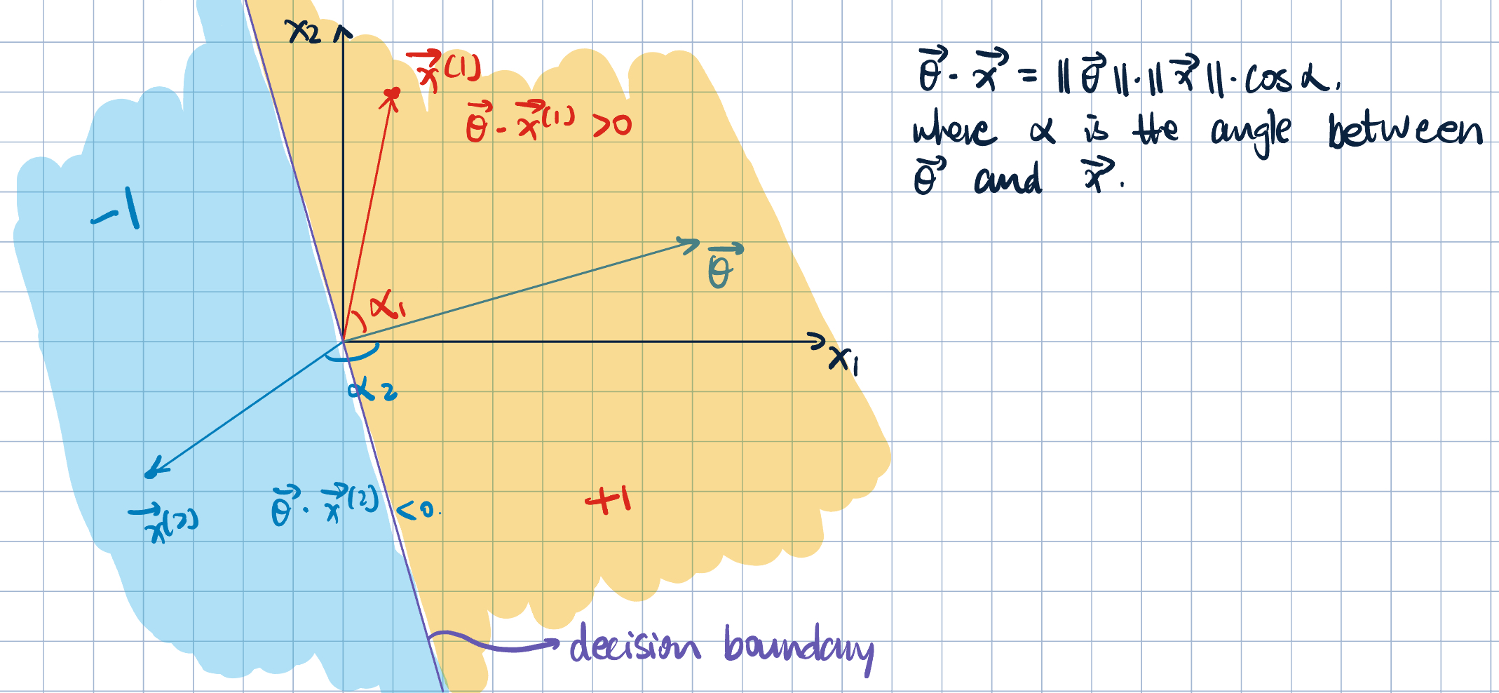
• However, what happens on this \(90^\circ\) line? We call this line the decision boundary, which separates the two classes. Recall: \[ \va\theta\cdot\va x=\norm{\va\theta}\cdot\norm{\va x}\cdot\cos 90^\circ=0. \]

• View the decision boundary as a hyperplane in \(\R^d\).

  • Does the length of \(\va\theta\) matter? No.
  • Does the direction of \(\va\theta\) matter? Yes.

Linear Classifier with Offset

Definition 2 (Linear Classifier with Offset) \[ h(\va x;\va\theta,b)=\operatorname{sign}(\va\theta\cdot\va x+b), \] where \(\va x\in\R^d\), \(\va\theta\in\R^d\), and \(b\in\R\). \(b\) is called the offset or intercept.

Graphical Representation

Figure 2: Linear Classifier with Offset

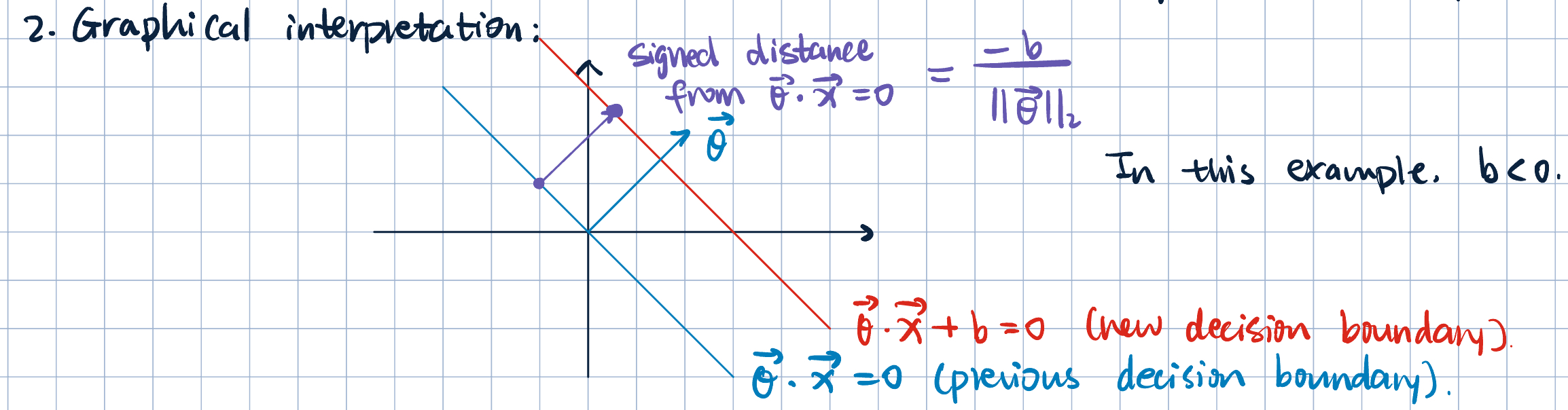
• Note that the signed distance from \(\va\theta\cdot\va x=0\) to the hyperplane \(\va\theta\cdot\va x+b=0\) is given by: \[ \dfrac{-b}{\norm{\va\theta}}. \]

Proof.

• Pick a point on old decision boundary \(\va x^{(1)}\) satisfies \[\va\theta\cdot\va x^{(1)}=0.\]
• Pick a point on the new decision boundary \(\va x^{(2)}\) satisfies \[\va\theta\cdot\va x^{(2)}+b=0\implies\va\theta\va x^{(2)}=-b.\]
• Let \(\va v=\va x^{(2)}-\va x^{(1)}.\)
• Now, project \(\va v\) into direction of \(\va\theta\): \[ \operatorname{proj}_{\va\theta}\va v=\qty(\va v\cdot\dfrac{\va\theta}{\norm{\va\theta}})\dfrac{\va\theta}{\norm{\va\theta}}. \] Note: \(\dfrac{\va\theta}{\norm{\va\theta}}\) is the unit vector in the direction of \(\va\theta\).
• Therefore, the signed sitance is given by: \[ \va v\cdot\dfrac{\va\theta}{\norm{\va\theta}}=\dfrac{\qty(\va x^{(2)}-\va x^{(1)})\cdot\va\theta}{\norm{\va\theta}}=\dfrac{\va x^{(2)}\cdot\va\theta-\va x^{(1)}\cdot\va\theta}{\norm{\va\theta}}=\dfrac{-b}{\norm{\va\theta}}. \]

Training Error

• Intuition: we want \(\va\theta\) that works well on training data \(D\).

Remark 1. We’ve restricted the class of possible clasassifiers to linear classifiers, reducing the chance of overfitting.

Definition 3 (Training Error and Learning Algorithms) The training error (\(\epsilon\)) is the fraction of training examples for which the classifier produces wrong labels: \[ \epsilon_N(\va \theta)=\dfrac{1}{N}\sum_{i=1}^N\1\qty{y^{(i)}\neq h\qty(\va x^{(i)};\va\theta)}, \] where \(\1\{\cdot\}\) returns \(1\) if true and \(0\) if false.

An equivalent form is: \[ \epsilon_N(\va \theta)=\dfrac{1}{N}\sum_{i=1}^N\1\{{\color{orange}{\underbrace{y^{(i)}\qty(\va\theta\cdot\va x^{(i)})}_{\substack{y^(i)\text{ and }\va\theta\cdot\va x^{(i)}\\\text{ have opposite signs}}}}}{\color{green}{\overbrace{\leq 0}^{\substack{\text{points on the decision boundary}\\\text{are considered misclassified}}}}}\} \]

• Goal: Find \(\displaystyle\va\theta^*=\argmin_{\va\theta}\epsilon_N\qty(\va\theta)\).
• How:
  • In general, this is not easy to solve (it’s NP-hard).
  • For now, we will consider a special case: linearly separable data.

Definition 4 (Linear Separable) Training examples \(D=\qty{\va x^{(i)}, y^{(i)}}_{i=1}^N\) are linearly separable through the origin if \(\exists\ \va\theta\) such that \[ y^{(i)}\qty(\va\theta\cdot\va x^{(i)})>0\quad\forall\ i=1,\dots, N \]

Remark 2. This assumption of linear separability is NOT testable.

Perceptron Algorithm

• The perceptron algorithm is a mistaken-driven algorithm. It starts with \(\va\theta=\va 0\) (the zero vector), and then tries to update \(\va\theta\) to correct any mistakes.

\begin{algorithm} \caption{Perceptron (Through Origin)} \begin{algorithmic} \Procedure{Perceptron}{$D=\qty{\va x^{(i)}, y^{(i)}}_{i=1}^N$} \State $k=0$; $\va\theta^{(0)}=\va 0$ \While{not all points are correctly classified} \For{$i=1,\dots, N$} \State \Comment{$\color{green}\text{if mistake}$} \If{$y^{(i)}\qty(\va\theta^{(k)}\cdot\va x^{(i)})\leq 0$} \State $\va\theta^{(k+1)}=\va\theta^{(k)}+y^{(i)}\va x^{(i)}$ \State $k++$ \EndIf \EndFor \EndWhile \EndProcedure \end{algorithmic} \end{algorithm}

Theorem 1 (Existence of Perceptron Solution) The perceptron algorithm (Algorithm 1) converges after a finite number of mistkaes if the training examples are linearly separable through the origin.

• However, :
  • Solution is not unique
  • May need to loop through the dataset more than once, or not use some points at all.

\begin{algorithm} \caption{Perceptron (With Offset)} \begin{algorithmic} \Procedure{Perceptron}{$D=\qty{\va x^{(i)}, y^{(i)}}_{i=1}^N$} \State $k=0$; $\va\theta^{(0)}=\va 0$; $b^{(0)}=0$ \While{not all points are correctly classified} \For{$i=1,\dots, N$} \State \Comment{$\color{green}\text{if mistake}$} \If{$y^{(i)}\qty(\va\theta^{(k)}\cdot\va x^{(i)}+b^{(k)})\leq 0$} \State $\va\theta^{(k+1)}=\va\theta^{(k)}+y^{(i)}\va x^{(i)}$ \State $b^{(k+1)}=b^{(k)}+y^{(i)}$ \State $k++$ \EndIf \EndFor \EndWhile \EndProcedure \end{algorithmic} \end{algorithm}

Proof. Produce augmented vecotrs: \[\va x'=\mqty[1, \va x]^\top\quad\text{and}\quad\va\theta'=\mqty[b,\va\theta]^\top.\] Then, we have implicit offset formula: \[\va\theta'\cdot\va x'=b+\va\theta\cdot\va x.\] Apply Algorithm 1 to \(\va x'\) and \(\va\theta'\): \[ \begin{aligned} \va\theta'^{(k+1)}&=\va\theta'^{(k)}+y^{(i)}\va x'^{(i)}\\ \mqty[b^{(k+1)},\va\theta^{(k+1)}]&=\mqty[b^{(k)},\va\theta^{(k)}]+y^{(i)}\mqty[1,\va x^{(i)}]\\ \implies \va\theta^{(k+1)}&=\va\theta^{(k)}+y^{(i)}\va x^{(i)}\\ b^{(k+1)}&=b^{(k)}+y^{(i)}. \end{aligned} \]